Build Dashboards and Kanban Boards with the Google Sheets Canvas Tool

With the new Sheets Canvas feature, we can build professional-looking interactive dashboards directly in our Google Sheets, using nothing more than natural language prompts. It’s a huge upgrade from how we used to build dashboards in Sheets.
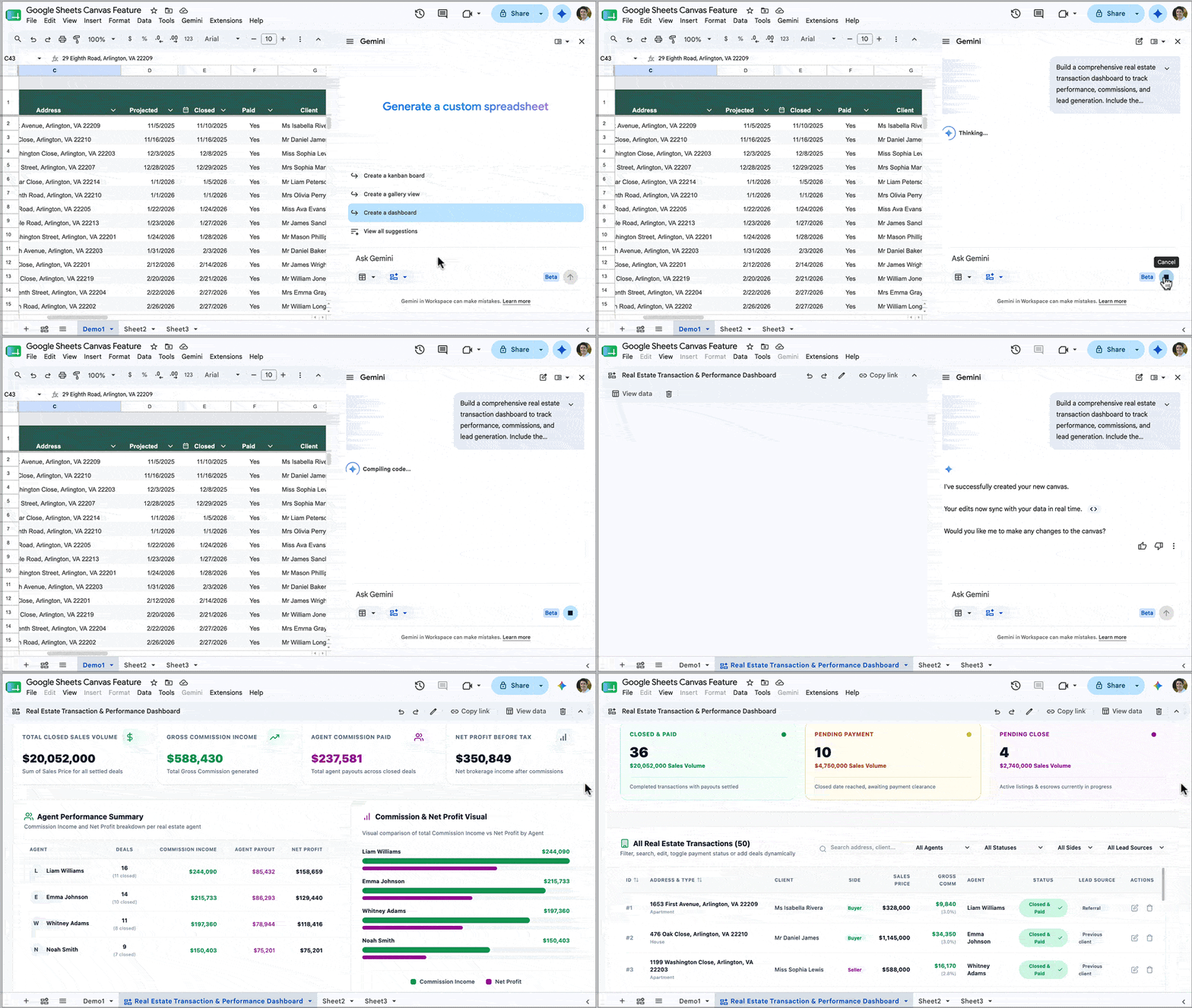
Sheets Canvas to build a professional dashboard

Previously, we clumped together charts and used formatting tricks such as borders and background cell colors to try and recreate a professional look. It was all rather challenging and time-consuming, with limited interactive options. (Read this post to see what I mean.)

Alternatively, we might have connected Google Sheets to a third-party tool, but these incurred extra costs, introduced security risks, and were often still pretty janky.

In this post, we are going to take a look at this new Sheets Canvas feature.

Sheets Canvas Availability

At the time of writing (August 2026), the Sheets canvas feature is only available to Google Workspace customers on Business or Enterprise Standard and Plus plans, or AI Pro for Education add-on subscribers, or to consumers on Google AI Pro and Ultra plans.

How To Build A Dashboard with Sheets Canvas

Firstly, you need to have your data ready to go in a Google Sheet, preferably in a Tables format, which is best for Gemini.

Secondly, it pays to think about your dashboard design before you start building it.

That way, you won’t end up building something that isn’t useful. Instead, you plan what information will be shown on the dashboard and how it will work, which will result in a more successful outcome.

For example, ask yourself these questions:

  • What are the key metrics to show?
  • Who is the intended audience for this dashboard?
  • How technically literate are they? Will they understand how to read complex charts?
  • How familiar are they with this data and its background context?

With your data and design plan to hand, you’re ready to start creating a Sheets Canvas.

There are three entry points:

  1. From the toolbar: Insert > Canvas
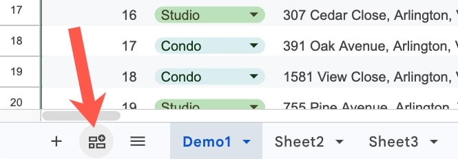
  2. Using the “Create a canvas” button in the bottom left of your Sheet, next to the Sheet names.
    (Both 1 and 2 open the Gemini sidebar with the Canvas option pre-selected.)
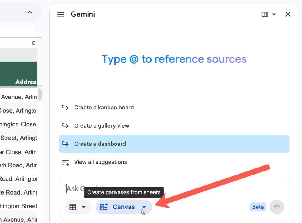
  3. You can select “Create canvas” directly in the Gemini sidebar too.

1. Insert menu:
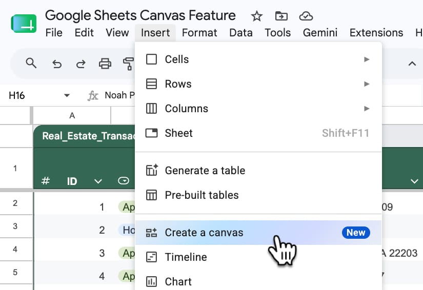
Toolbar menu to insert a Sheets Canvas

2. Create a canvas button:

Insert button for Canvas feature in Google Sheets

3. Create canvas in Gemini Sidebar:

Canvas feature in Gemini sidebar of Google Sheet

With Gemini sidebar open and the canvas feature selected, make sure you select the correct dataset(s) for the dashboard.

Use the button next to the Canvas option and choose the sheet containing your data. If you already have that sheet open, then it will automatically be selected, and you can deselect the other sheets if you don’t need them.
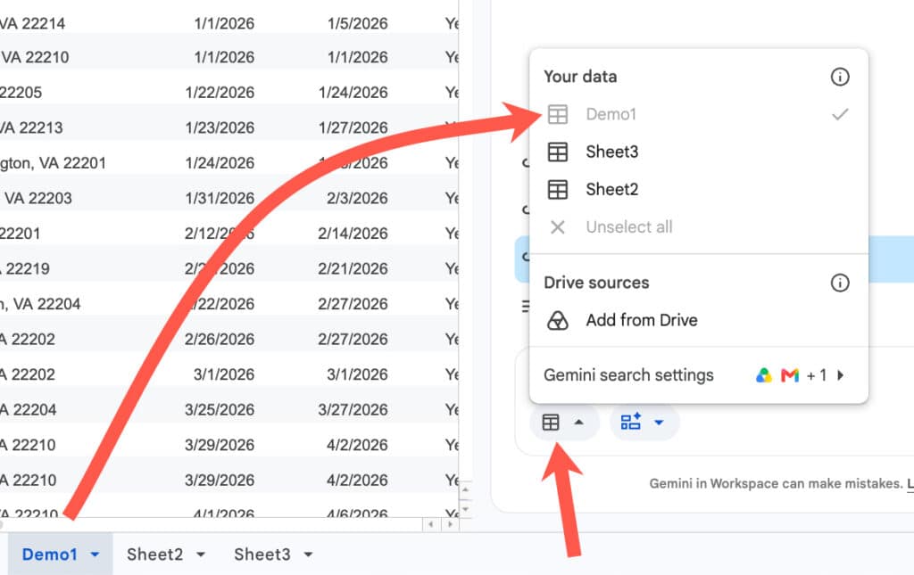
Select data in Sheets Canvas

Now you’re ready to insert your prompt.

Example 1: Real Estate Dashboard

Consider this dataset of real estate transactions:
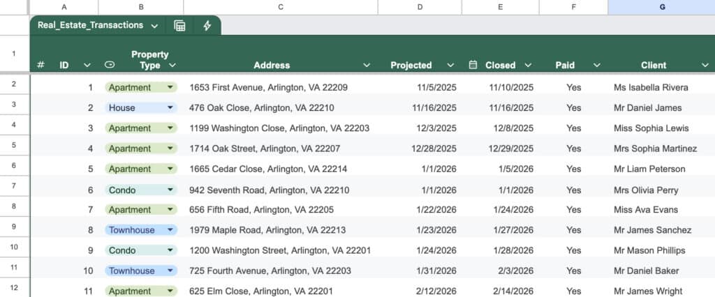
Real Estate data in Google Sheets

Here’s an example prompt to build a dashboard for this data:

Build a comprehensive real estate transaction dashboard to track performance, commissions, and lead generation. Include the following elements:

1. Key Performance Indicators (KPIs): Calculate the total sum of Sales Price, Commission Income, Agent Commission, and Net Profit for Tax for all “Closed” and “Paid” deals.

2. Agent Performance: Create a summary table or chart showing the total Commission Income and Net Profit generated by each Agent.

3. Lead Source Analysis: Create a bar chart breaking down total Sales Price and total number of transactions by Lead Source to see which marketing channels are most effective.

4. Buyer vs. Seller Split: Create a visual breakdown comparing the number of transactions and total Commission Income based on the Deal Side (Buyer vs. Seller).

5. Deal Pipeline: Provide a quick count of transactions categorized by Deal Status to show how many deals are currently pending versus closed.

Please format this with a clean, professional layout, using bold headers for each section and placing the charts logically next to the summary tables. 

Use hex color #0F9E59 as the primary color and #9E0F9C as the secondary color.

Pro Tip: Save your best dashboard prompts in a prompt library for future reuse.

Typically, Gemini takes a few minutes to build the dashboard, depending on how complex your prompt is.

The output for the real estate data example looks like this:
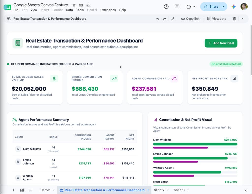
A real estate dashboard built using Google Sheets Canvas

Notice how the colors match the colors mentioned in the prompt (#0F9E59 as the primary color and #9E0F9C as the secondary color).

Also, notice the “Add New Deal” button in the top right corner. When you click this, it opens a pop-up with a form to add new deals:
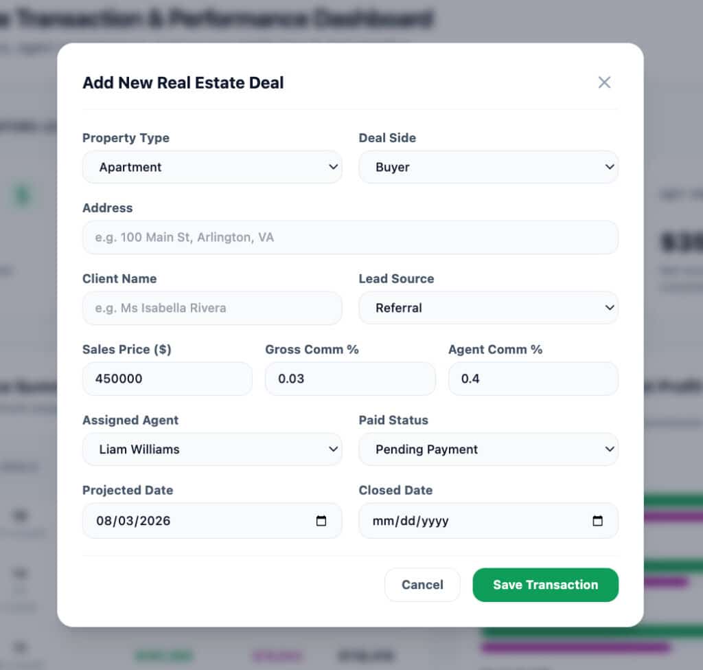
Add new data button in Sheets Canvas

This data is inserted directly into your original data table in Google Sheets. It’s a great way for users to add new data without leaving the dashboard view, and it saves users from needing to navigate the data in the spreadsheet itself.

At the the top of the canvas is a small edit bar for making changes, sharing, or deleting the canvas:

To use the “Copy link” button to share the canvas, you need to first grant file access (through the regular “Share” button in the top right of your Google Sheet) to anyone you want to share the canvas with.

Example 2: Kanban Board

The Sheets canvas tool is not limited to regular dashboards, though.

It can also build interactive Kanban boards, which is my favorite use case and a killer feature.
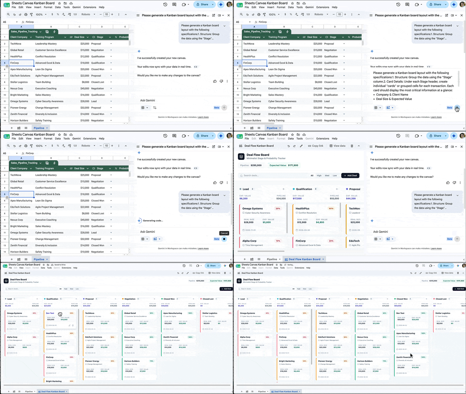
Build a Kanban board in Google Sheets with the Canvas feature.

Kanban boards are visual project management tools that organize tasks into columns and allow you to drag and drop cards between these columns.

Previously, this sort of interactivity was impossible inside of Google Sheets, but now with this new Sheets Canvas feature, you can build a fully featured Kanban board with a single prompt.

For example, here is a client pipeline data set for training contracts:
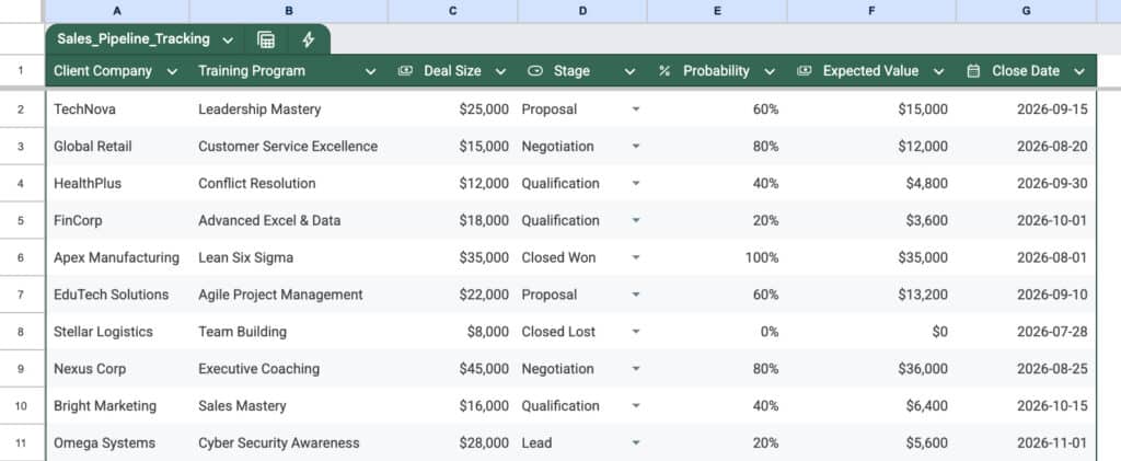
Sales Data Pipeline in Google Sheets

And here’s an example prompt to generate a Kanban board from this data:

Please generate a Kanban board layout with the following specifications:

1. Structure: Group the data using the “Stage” column.

2. Card Details: Under each Stage header, create individual “cards” or grouped cells for each transaction. Each card should display the most critical information at a glance:

  • Company & Client Name
  • Deal Size & Expected Value

3. Formatting:

  • Please apply conditional formatting or color-coding to the cards based on the “Probability” column (e.g., green for high probability, yellow for medium, red/gray for low) so I can easily identify which deals are most likely to close.
  • Ensure the layout is clean and minimalist.

The output from this prompt looks something like this:
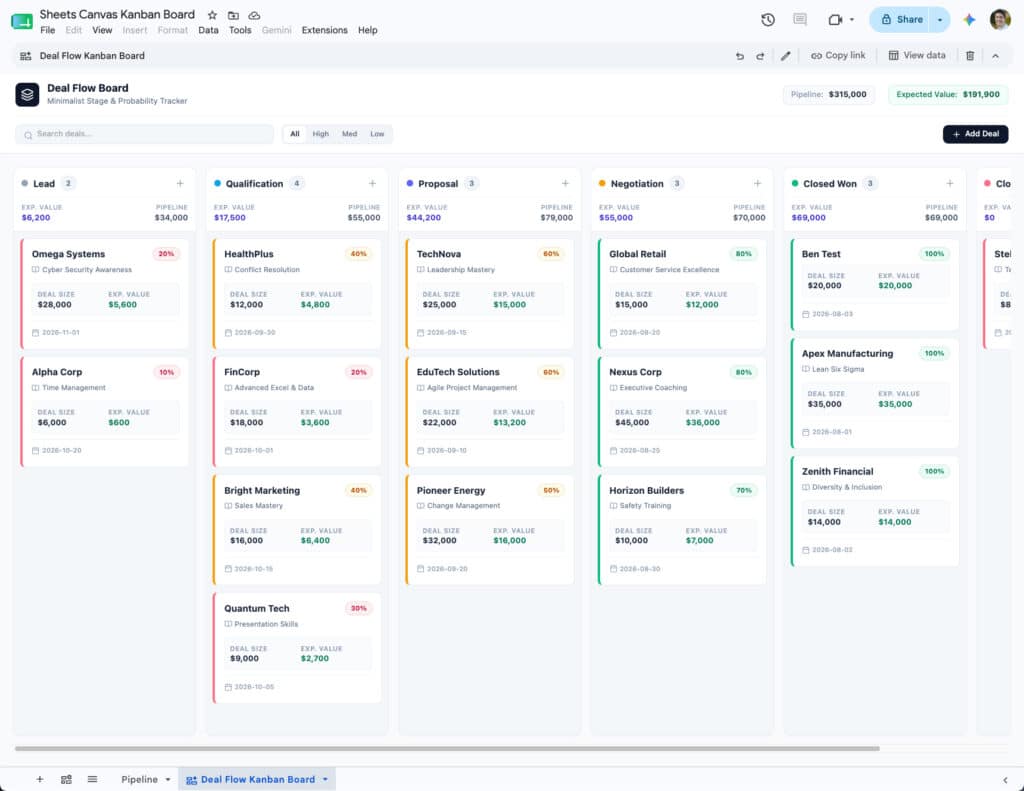
Kanban Board in Sheets Canvas

You can then drag these cards into different columns as needed to show progress. When you drag a card into a new column, the data in the underlying sheet also updates to reflect that, so they are always synced in real time.

And as with the dashboard from earlier, there is also a button to add new data from the Kanban canvas rather than having to go back to the actual spreadsheet data.

Limitations

At the moment, if you want to modify the dashboard generated by the Sheets Canvas tool, you give it an additional prompt in the Gemini sidebar. For example, you might prompt Gemini with “change the leads pie chart into a bar chart“.

Unfortunately, when Gemini updates the dashboard, other elements might inadvertently change too.

I think the real breakthrough will come when we can click on individual features within the Dashboard or Kanban board and give specific instructions to modify that specific feature only with a prompt. Hopefully that is something coming down the line.

Conclusion

This new Sheets Canvas feature is a fantastic tool that dramatically expands the possibilities of what you can do with data in Google Sheets.

And, whilst the regular chart tool will remain extremely useful for specific analysis and one-off charts, the old way of building dashboards is rapidly becoming obsolete.

I can’t imagine spending hours manually positioning charts, hand-picking background cell colors and borders, and all manner of other dark arts, to build a dashboard the old way, knowing it wouldn’t even look half as good as what this new canvas tool can build in a few minutes.

If you have access to this canvas tool, then I encourage you to experiment with it to build your dashboards.
11 Incredibly Useful URL Tricks for Google Sheets

Did you know that by changing the URL of a Google Sheet we can change how it behaves?

In this post, we look at 11 incredibly useful URL Tricks for Google Sheets.

For example, we can create a URL that automatically downloads the Sheet as a PDF. Or create a template ready for copying. And much more.

URL Tricks for Google Sheets

Take a look at any Google Sheets URL in the address bar of your browser.

It will take the following form:

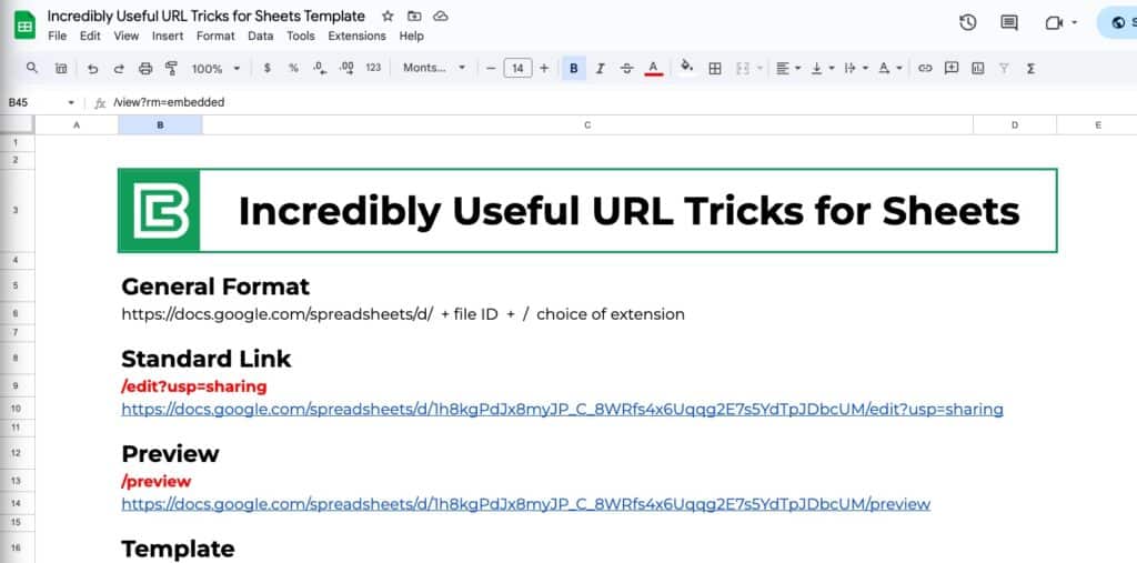
https://docs.google.com/spreadsheets/d/ + file ID + / extension

We can change the /extension at the end of the URL to ensure a different action happens when a user uses that URL.

Feel free to click on any of the links below to see how they work. They are all linked to the following template, which you can copy for your own reference (bonus points if you use the correct URL trick to do that).

URL Tricks for Google Sheets

1. Standard Sharing Link Format

This is the default sharing link for Google Sheets. Users with appropriate permissions can view or edit the sheet.

  • Advantages: Provides direct access to the Sheet with full functionality.
  • Limitations: If set to “Anyone with the link can edit,” any users can make changes.
  • Best For: Team collaboration when you want users to view or edit the Sheet.

Extension Format:
/edit?usp=sharing

Example link:
https://docs.google.com/spreadsheets/d/1h8kgPdJx8myJP_C_8WRfs4x6Uqqg2E7s5YdTpJDbcUM/edit?usp=sharing

2. Preview

Opens the spreadsheet in a read-only format without showing the editing toolbar.

  • Advantages: Cleaner presentation without distractions from menus and tools.
  • Limitations: Users cannot edit or copy directly from this view.
  • Best For: Great for sharing data in a presentation format when you don’t want users to make edits.

Extension Format:
/preview

Example link:
https://docs.google.com/spreadsheets/d/1h8kgPdJx8myJP_C_8WRfs4x6Uqqg2E7s5YdTpJDbcUM/preview​

3. HTML View

Converts the sheet into a basic HTML page.

  • Advantages: Loads faster and is accessible without needing Google Sheets’ interface.
  • Limitations: Some formatting and interactive features may not function properly.
  • Best For: Useful for reports since it eliminates sheet controls but allows you to still navigate between tabs.

Extension Format:
/htmlview

Example link:
https://docs.google.com/spreadsheets/d/1h8kgPdJx8myJP_C_8WRfs4x6Uqqg2E7s5YdTpJDbcUM/htmlview

4. Template

Opens a “Use Template” preview, allowing users to see and create their own copy of the file.

  • Advantages: Prevents accidental changes to the original document while ensuring consistency across copies.
  • Limitations: Users must have permission to access the original file.
  • Best For: Ideal for distributing Google Sheets to wider audiences so they can create their own copies.

Extension Format:
/template/preview

Example link:
https://docs.google.com/spreadsheets/d/1h8kgPdJx8myJP_C_8WRfs4x6Uqqg2E7s5YdTpJDbcUM/template/preview​

5. Make a Copy

Prompts users to create their own editable copy of the spreadsheet.

  • Advantages: Ensures the original file remains unchanged and user makes a copy.
  • Limitations: Requires users to be signed into Google to create a copy.
  • Best For: Useful for ensuring users make a copy of a Google Sheet.

Extension Format:
/copy

Example link:
https://docs.google.com/spreadsheets/d/1h8kgPdJx8myJP_C_8WRfs4x6Uqqg2E7s5YdTpJDbcUM/copy​

6. Export as a PDF

Generates a downloadable PDF version of the spreadsheet.

  • Advantages: PDF format ensures consistency across devices and prevents edits.
  • Limitations: Not interactive, not all features will display correctly; updates to the sheet require generating a new PDF.
  • Best For: Perfect for distributing static reports, tables, invoices, or finalized documents.

Extension Format:
/export?format=pdf

Example link:
https://docs.google.com/spreadsheets/d/1h8kgPdJx8myJP_C_8WRfs4x6Uqqg2E7s5YdTpJDbcUM/export?format=pdf​

7. Export as a CSV

Provides a downloadable CSV version of the sheet, exporting only the active tab.

  • Advantages: Downloads your data in a universal format compatible with most data processing tools.
  • Limitations: Loses formatting, formulas, interactive elements, and multiple sheet structures.
  • Best For: Great for exporting data tables for analysis in other software, such as databases or coding environments.

Extension Format:
/export?format=csv

Example link:
https://docs.google.com/spreadsheets/d/1h8kgPdJx8myJP_C_8WRfs4x6Uqqg2E7s5YdTpJDbcUM/export?format=csv​

8. Export as an Excel Document

Downloads the spreadsheet as an Excel (.xlsx) file.

  • Advantages: Retains formulas, formatting, and multiple sheets.
  • Limitations: Some Google Sheets-specific features (like QUERY function or Google Apps Script) may not work in Excel.
  • Best For: Best for sharing Sheets with users who prefer or require Excel.

Extension Format:
/export?format=xlsx

Example link:
https://docs.google.com/spreadsheets/d/1h8kgPdJx8myJP_C_8WRfs4x6Uqqg2E7s5YdTpJDbcUM/export?format=xlsx​

9. Distraction Free Editor

Opens the sheet in a minimalistic mode with no toolbars or menus.

  • Advantages: Reduces clutter and distractions for focused editing.
  • Limitations: Some editing options may not be accessible.
  • Best For: Useful for presenting data cleanly or working in a distraction-free environment.

Extension Format:
/view?rm=minimal

Example link:
https://docs.google.com/spreadsheets/d/1h8kgPdJx8myJP_C_8WRfs4x6Uqqg2E7s5YdTpJDbcUM/view?rm=minimal​

(Because I shared a view-only copy, you won’t be able to do any editing. Share with editor rights if you want to use this feature.)

10. Basic Controls Editor

Opens the sheet in a limited interface with only essential tools.

  • Advantages: Allows basic editing without overwhelming users.
  • Limitations: Lacks full editing capabilities.
  • Best For: Ideal for users who need to make small modifications but don’t require full spreadsheet features.

Extension Format:
/view?rm=demo

Example link:
https://docs.google.com/spreadsheets/d/1h8kgPdJx8myJP_C_8WRfs4x6Uqqg2E7s5YdTpJDbcUM/view?rm=demo​

11. Embed in Iframe

Embeds the spreadsheet in a webpage without extra Google Sheets UI elements.

  • Advantages: Provides a seamless way to display live data in a website or online dashboard.
  • Limitations: Users cannot interact fully unless given editing access.
  • Best For: Great for embedding spreadsheets in blogs, dashboards, or reports where live data needs to be displayed.

Extension Format:
/view?rm=embedded

Example link:
https://docs.google.com/spreadsheets/d/1h8kgPdJx8myJP_C_8WRfs4x6Uqqg2E7s5YdTpJDbcUM/view?rm=embedded​

Multiple Selections in Drop Downs in Google Sheets

The drop down menu feature in Google Sheets is useful for efficient data entry. It can also be used to create dynamic spreadsheets, for example, dashboards that change based on choices a user makes.

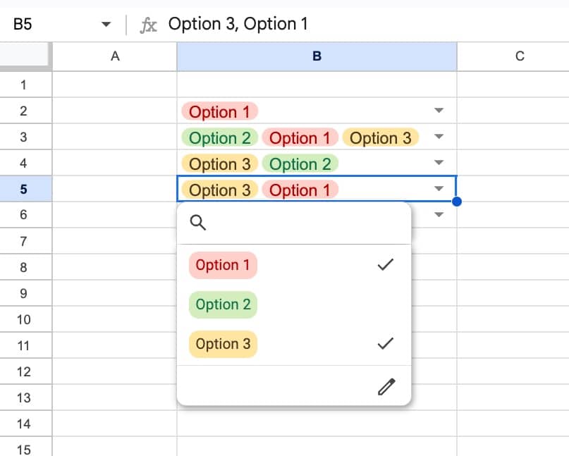
At the end of July 2024, Google announced multiple selections in drop downs (scheduled to roll out in late-August/early-September). This is great news that will give us even more flexibility in our spreadsheets.

In this post, we’re going to take a look at this new drop down feature:

Multiple Dropdowns in Google Sheets

How to Enable Multiple Selections in Drop Downs

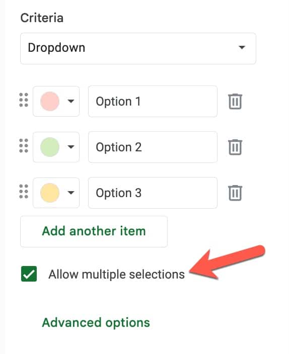
To enable multiple selections, create a regular dropdown and then check the box that says “Allow multiple selections”:

Allow Multiple Selections in Google Sheets dropdown

Boom! 💥 That’s it.

Working with Drop Down Multiple Selections in Formulas

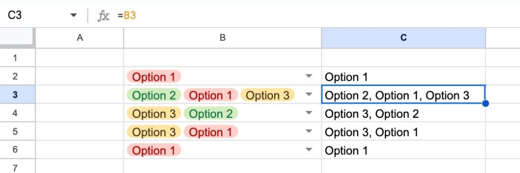
If you select multiple options from a drop down menu, the output is a comma separated list:

Multiple Selections in Drop Downs in Google Sheets

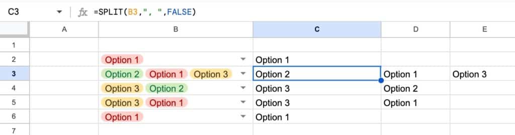
To work with them in formulas, we use the SPLIT function to separate the choices into their separate parts.

Note the space after the comma. We need to be mindful of this in our formulas. Split out the comma-separated lists with this formula, which accounts for the space too:

=SPLIT(B2,", ",FALSE)

It looks like this in our Sheet:

Split formula for multiple Dropdowns

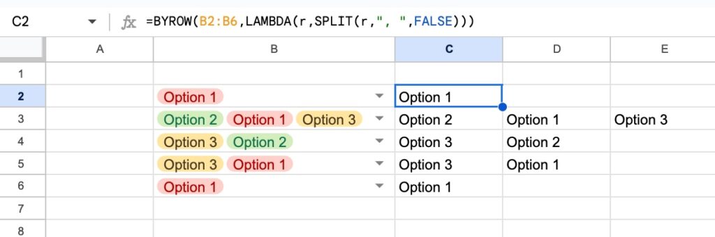
We can use a BYROW function to expand this SPLIT formula to work with a range of multi dropdowns. This single formula in cell C2 splits out all the cells in the range B2:B6 and outputs all the data in C2:E6 range:

=BYROW(B2:B6,LAMBDA(r,SPLIT(r,", ",FALSE)))

In our Sheet:

BYROW and SPLIT with multiple dropdowns

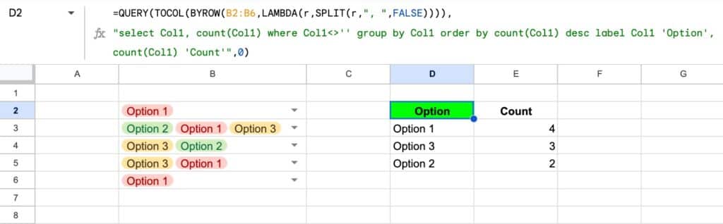
Finally, we could wrap this with a TOCOL function and a QUERY function to count our choices:

=QUERY(TOCOL(BYROW(B2:B6,LAMBDA(r,SPLIT(r,", ",FALSE)))),
"select Col1, count(Col1) where Col1<>'' group by Col1 order by count(Col1) desc label Col1 'Option', count(Col1) 'Count'",0)

In our Sheet:

Multiple Selections in Drop Downs with QUERY

GETPIVOTDATA Function in Google Sheets: How To Extract Data From Pivot Tables

The GETPIVOTDATA function is used to extract data from a pivot table.

Pivot tables are one of the most powerful and useful features in spreadsheets. We use them to summarize our data, by grouping, sorting and filtering it.

But pivot tables are dynamic elements. That means they can change size and shape when data is added or removed from the underlying dataset (e.g. when a new category is added). This makes it tricky to extract data consistently.

When a pivot table changes size, a regular cell reference (e.g. A12 or F34) might not point to the correct value in the pivot table anymore. However, the GETPIVOTDATA function will still extract the correct data.

The downside of GETPIVOTDATA is that it’s fiendishly difficult to use. It’s something of a dark art to identify the correct rows and columns inside the function.

In this post, we’re going to learn how this function works.

👇 Feel free to grab the template from the bottom of this article to follow along.
Continue reading GETPIVOTDATA Function in Google Sheets: How To Extract Data From Pivot Tables

The Complete Guide to Tables in Google Sheets


28 Days to Gemini Mastery

New course

Stop dabbling with Gemini. Start building AI systems.

One-off prompts → repeatable workflows Gemini across all your Workspace tools
Automations and agents that save hours NotebookLM, vibe coding, Gemini Gems

In this post, we’re looking at the new, powerful Tables in Google Sheets.

We’ll start with the basic benefits and features of Tables. Then we’ll look at how you can work with data with Tables using the new Views feature. After that, we’ll look at how to use Tables with formulas and structured table references.

Tables In Google Sheets Animation

What are Tables in Google Sheets?

Tables are a new feature in Google Sheets. They make it quick and easy to apply formatting and structural rules to a plain range of data.

There are a lot of benefits to using Tables to work with data (see below). I’m excited to use Tables in my Sheets workflows, especially the new Group By views.

Why should you use Tables?

There are many benefits to using Tables, including:

  • Quick and easy to apply formatting
  • Header row is automatically locked at the top of the Table
  • Nice selection of pre-built Table templates
  • Nice selection of pre-built styles
  • Super easy to add dropdowns or smart chips to columns
  • Formulas automatically applied down whole column
  • Formatting and calculations are applied automatically to new rows
  • Super easy access to filter and group by views
  • Some folks will love the Structured Table formula referencing
  • Built-in data validation with the column datatypes

When should you not use Tables?

Like any spreadsheet technique, Tables won’t be the best choice for every situation:

  • Tables might be confusing to people who are unfamiliar with them
  • They introduce additional complexity and clutter to Sheets that you might not want
  • The structured Table reference formulas can be confusing to the uninitiated
  • They work best with uniform underlying data. If your data has blank rows, subtotals, etc. then Tables may not interpret it correctly
  • It’s sometimes not possible to convert large, complex datasets into Tables

Tables Basics

Pre-Built Tables

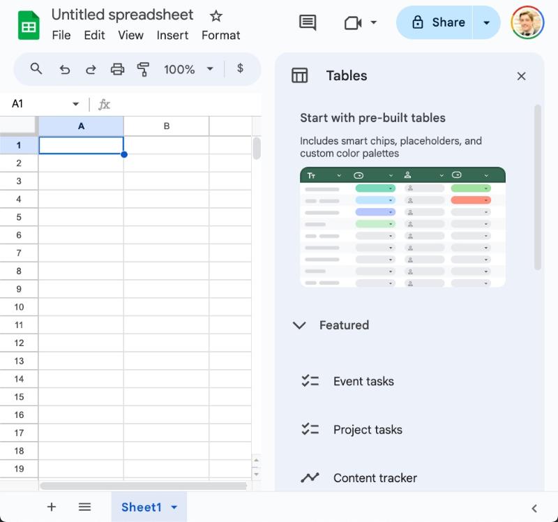
Currently, when we open a new Google Sheet, we’re prompted to create a new Table with the Pre-Built Tables sidebar:

Pre-Built Tables in Google Sheets

Using this, we can insert a pre-built table with a single click.

I doubt this will always open by default. It’s a deliberate choice to expose more people to Tables since they’re a new feature.

I see this being very helpful for people earlier in their Sheets journey. It showcases some of the best features — dropdowns, smart chips, etc. — that many folks don’t know about.

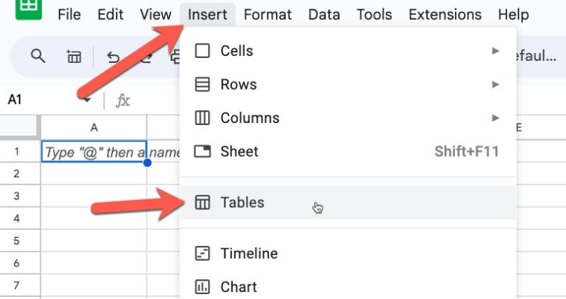
Access the Pre-Built Tables sidebar from the menu: Insert > Tables

Insert Tables in Google Sheets

How to create Tables in Google Sheets

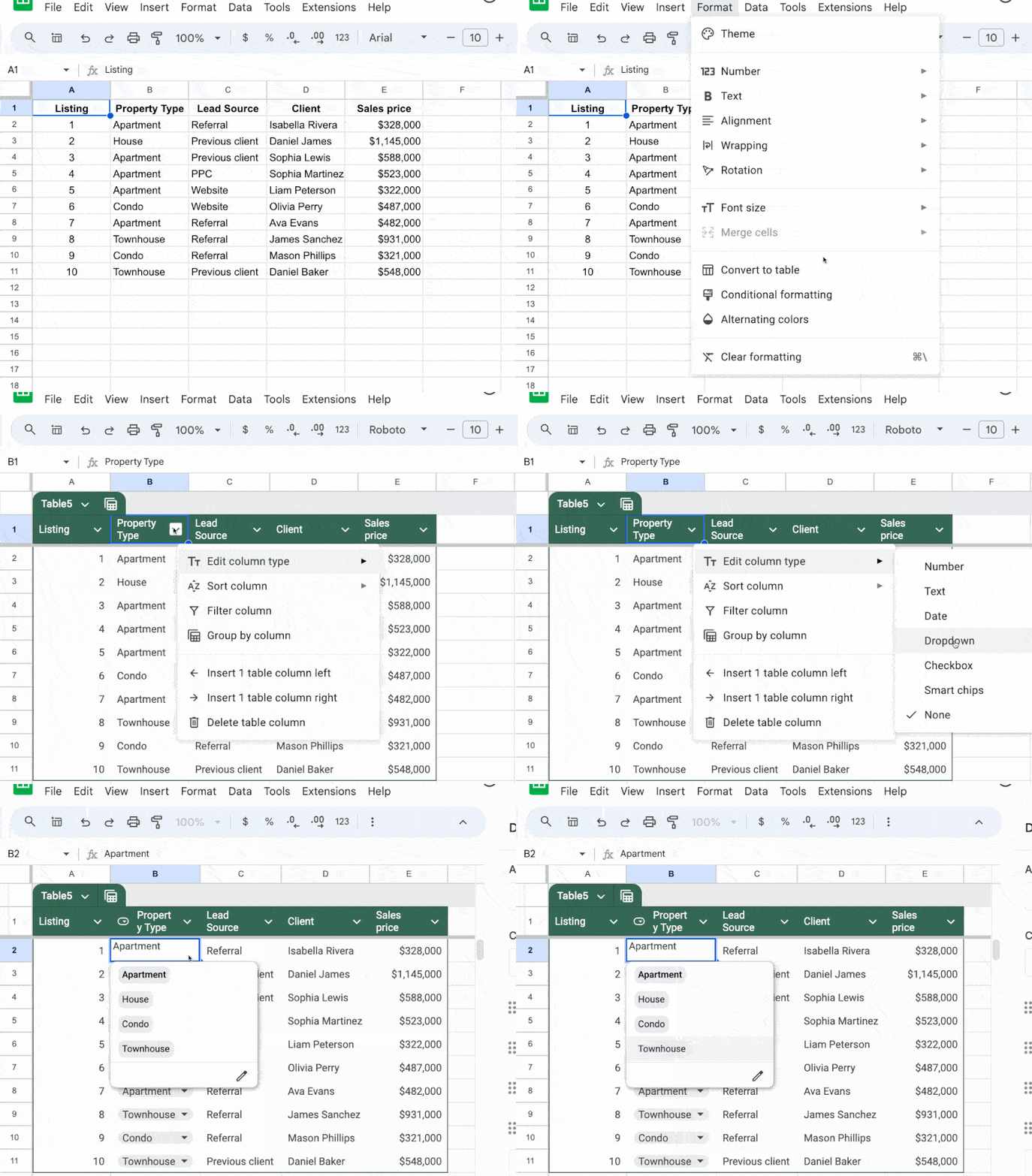
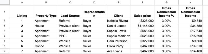
Now, suppose we already have this dataset in our Sheet:

Data in Google Sheets

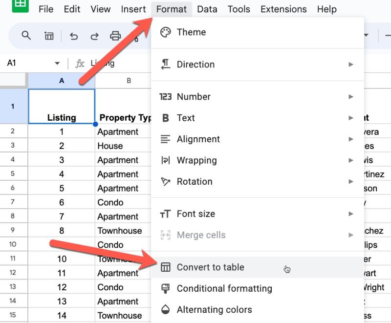
Click on any cell in a dataset and convert it to a Table via this menu:

Format > Convert to table

Format menu in Google Sheets

The new Table looks like this:

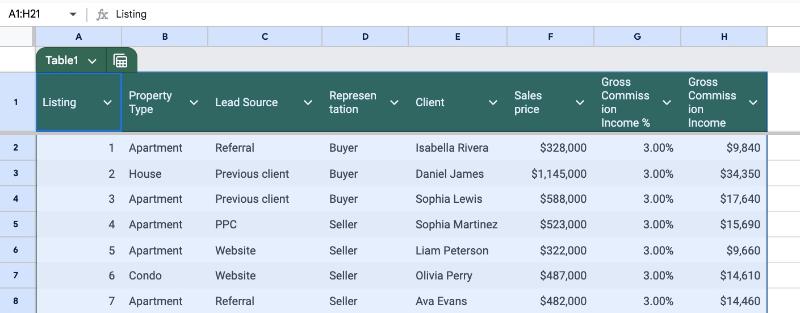
Tables in Google Sheets

Now we can enjoy all the benefits of Tables that we mentioned above!

The main Table Menu

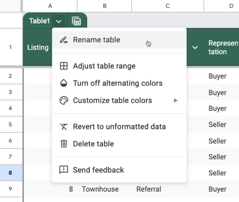
Table Menu in Google Sheets

Click on the down arrow next to the Table name in the top left corner of the Table to open the Table menu.

From this menu, we can rename the Table, change the formatting, apply custom formats, or even delete the Table.

Be warned: Deleting the Table also deletes the underlying dataset. Use the “Revert to unformatted data” if you want to return to your base data.

The Column Menu

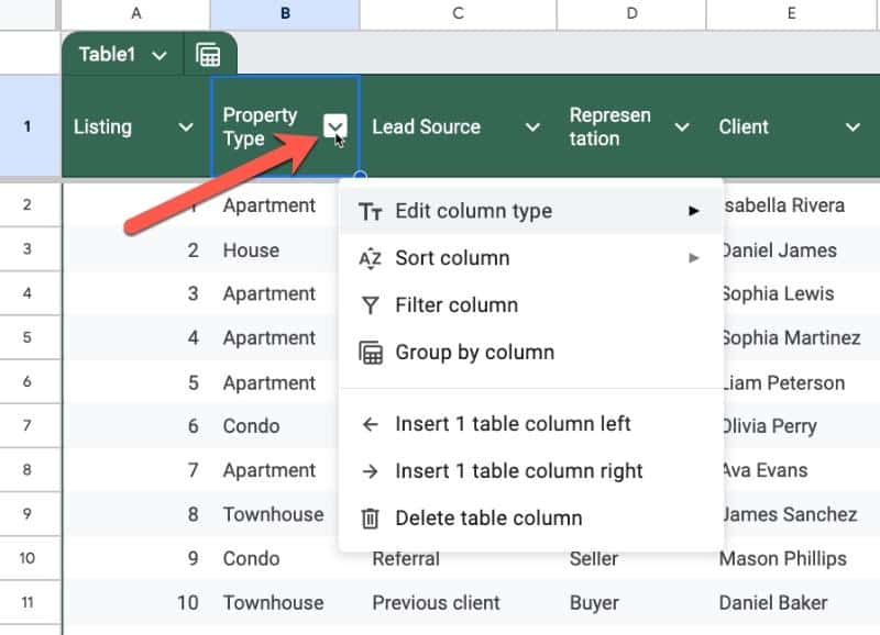
Column Menu in Tables feature of Google Sheets

Click on the down arrow next to each column heading to open the Column Menu for that column.

Here, we can set the datatype for the column (i.e. is it text? A number? A smart chip?). This is a powerful setting so worth taking time to get to know.

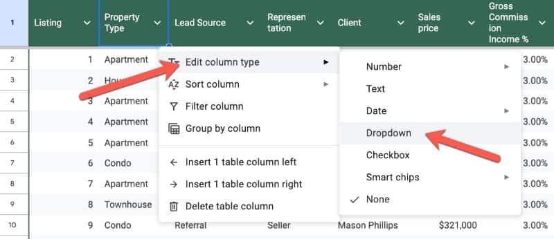
For example, we can set a column to dropdown type and it will convert the entire column in a single click.

Dropdown option in Google Sheets Tables

We can also filter and group by columns, which we discuss below.

And, there’s an easy way to add or remove columns from this column menu.

Data Analysis Tools Within Tables

One of the main benefits to using Tables with our datasets is the built-in data analysis tools that we get.

Built-in Data Validation

Setting column types can feel like an additional burden, but there are benefits.

One of the main benefits is the automatic data validation it provides.

Here’s how it works.

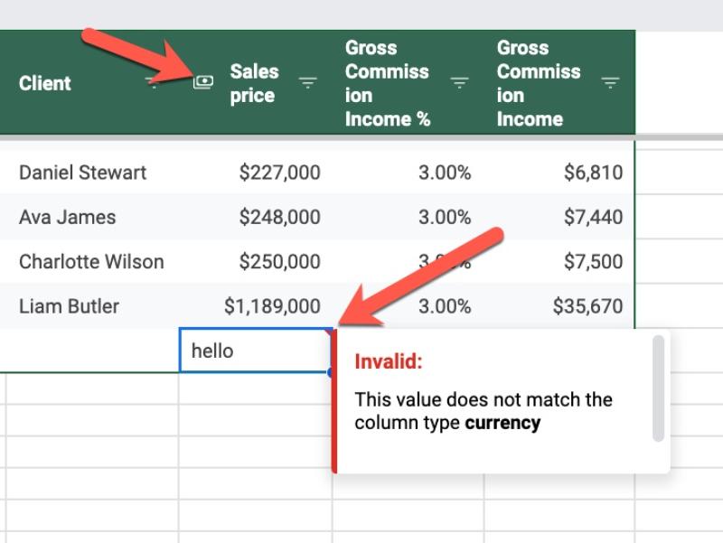
Suppose we set our column to be a Currency type column. This is shown by a small icon next to the column name (the first red arrow).

Then along comes a colleague who enters a new row. But they accidentally type a name (or other word) into that number column.

The Table will add a red warning flag and error message to indicate invalid data in that column:

Data validation in Tables in Google Sheets

Table Views Menu

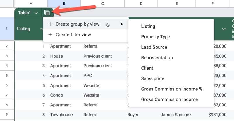
The Table Views menu is accessed from the Table icon next to the Table name, in the top left of the Table:

Table Views Menu in Google Sheets

Opening the Table view menu lets us create Group By or Filter Views, or access previously built views.

Group By Views

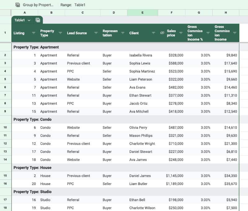
The new Group By View aggregates data into categories based on a selected column.

For example, we could group our data by property type with Group By View so that we can see all the groups together:

Group By Views in Google Sheets Tables

(One feature that is lacking with Group By Views is subtotal values for these groups. Fingers crossed we’ll get this in the future.)

Group By views can be created from either the Table View menu or from the selected Column menu.

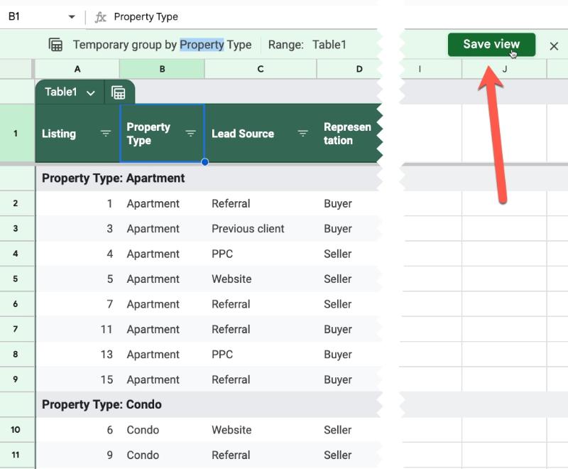
To save a View (Group By or Filter) click on the “Save view” button:

Save View in Google Sheets Tables

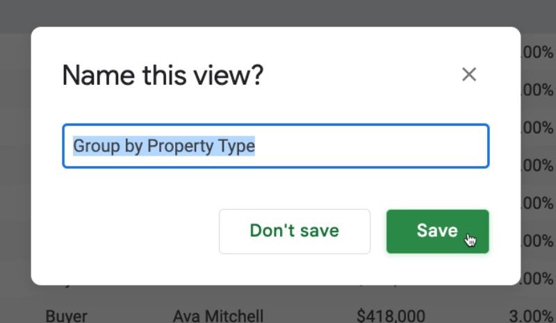
Give the view a name in the subsequent popup:

Name this view in Google Sheets Tables

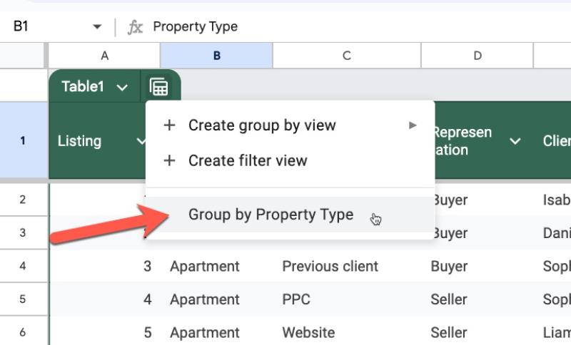
Now, this view will always be accessible from the main Table Views menu:

Group By View in Tables menu

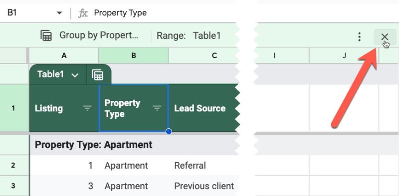
To close a view and return to the main Table view, press the “x” button on the right side of the green view bar between the formula bar and the Sheet.

Close button for Table view

Tables Filters

Filters are a HUGELY useful tool for exploring our data. They let us select subsets of data to review, based on categories (e.g. all the records for Client A) or conditions (e.g. all values over $100).

But many people aren’t aware they exist or forget to use them.

With Tables, they are applied automatically so that we can start using them immediately.

Access the Filter options inside the Column menu.

Tables Filter Views

Suppose we create a specific filter (all transactions with Client A over $100 in value) that we want to review over and over. Or share easily with colleagues.

We can create a Filter view and save this particular set of filter conditions to return to in the future.

Formulas In Tables

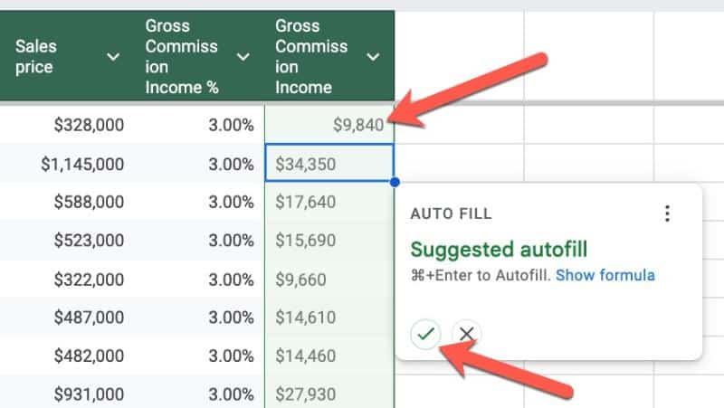
If you add a formula to the first row of a Table, you’re prompted to fill the entire column with Suggested Autofill:

Autofill Column in Table Google Sheets

(Note: This is the same behavior as regular non-Table formatted data.)

Table Reference Syntax

Table References are a special way to access data inside a Table. Instead of A1-style cell references, we can use the Table name and Column headings in our formulas.

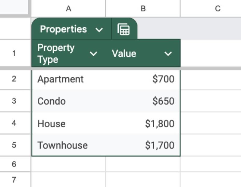
Let’s use this simple Table to illustrate the Table Referencing syntax:

Tables in Google Sheets

I’ve named this Table Properties.

(Note: Table names can only contain letters and numbers and can’t start with a digit or have a space.)

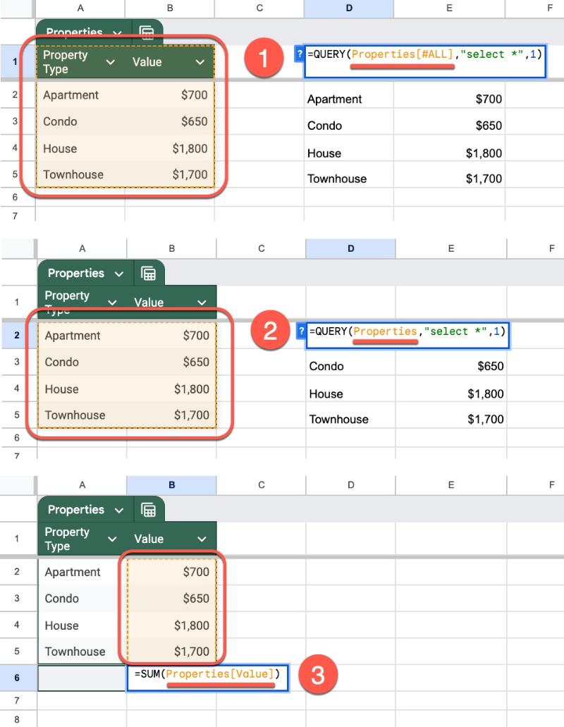
Here’s how the Table Referencing works:

  1. Properties[#All] –> entire Table AND column headers
  2. Properties –> gets Table data only, NO column headers
  3. Properties[Column Name] –> gets data in named column only

(Note: column heading names CAN contain spaces, but must be unique within that Table.)

It’s easier to understand visually and I’ve added formulas to show how they work:

Table References in Google Sheets

If you’re familiar with ​Named Ranges​, then you’ll feel right at home using Table referencing.

(Note: you can still access cells inside Tables using regular cell references, e.g. =A1.)

Benefits of using Table References

There are a number of benefits to using Table References over standard A1-style cell references:

  • The formulas automatically update to include any new rows of data added to the Table
  • If you create, rename, insert, or delete columns in a Table, any Table References in formulas will automatically update too
  • Easier to create than regular cell references. It’s easier to type “Properties[Value]” than e.g. “Sheet6!B2:B6”
  • When you start typing a Table or Column name, the auto-complete box will show any Table References that you can quickly click

Using Table References in Formulas

Now we understand structured table references, let’s see them in action with a practical example.

Let’s say we have a Table of real estate transactions. We call it RealEstate2024 (remember, no spaces allowed in Table names).

Now suppose we want to lookup a client name from that Table to retrieve transaction details.

To do that, we’ll use an ​XLOOKUP formula​.

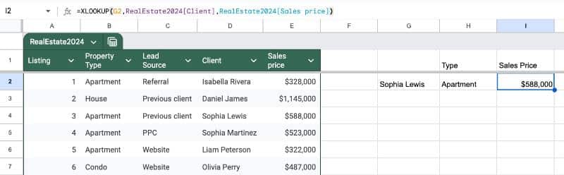
With our search term in cell G2 and using Table References, our formula is:

=XLOOKUP( G2 , RealEstate2024[Client] , RealEstate2024[Sales price] )

RealEstate2024[Client] refers to the “Client” column inside the “RealEstate2024” Table. Similarly, RealEstate2024[Sales price] refers to the “Sales price” column inside that same table.

In our Sheet, it might look like this:

Table References in Google Sheets

And here’s the equivalent A1-style formula:

=XLOOKUP( G2 , 'Copy of Sheet4'!D2:D21 , 'Copy of Sheet4'!E2:E21 )

The Table Reference version is definitely cleaner and easier to understand.

Plus, any new rows of data added to the Table will be automatically included by the formula. Whereas, with the A1-style formula, we’ll need to remember to update the range references.

Now, I’m not about to tell you that you can throw away your A1-style referencing!

Tables References are super useful and worth using if you have your data in a Table. However, A1-style references are more flexible and still necessary for more complex formulas.

Further Resoures

Tables Documentation from Google