Spreadsheets Archives - Page 19 of 35 -

The FACT Function in Google Sheets (And Why A Shuffled Deck of Cards Is Unique)

Let’s start with a mind-blowing fact, and then use the FACT function in Google Sheets to explain it.

Pick up a standard 52 card deck and give it a good shuffle.

The order of cards in a shuffled deck will be unique.

One that has likely never been seen before in the history of the universe and will likely never be seen again.

I’ll let that sink in.

Isn’t that mind-blowing?

Especially when you picture all the crazy casinos in Las Vegas.

Let’s understand why, and in the process learn about the FACT function and basic combinatorics (the study of counting in mathematics).

Four Card Deck

To keep things simple, suppose you only have 4 cards in your deck, the four aces.

You can create this deck in Google Sheets with the CHAR function:

The formulas to create these four cards are:

Ace of Clubs:

=CHAR(127185)

Ace of Spades:

=CHAR(127137)

Ace of Hearts:

=CHAR(127153)

Ace of Diamonds:

=CHAR(127169)

Let’s see how many different combinations exist with just these four cards.

Pick one of them to start. You have a choice of four cards at this stage.

Once you’ve chosen the first one, you have three cards left, so there are 3 possible options for the second card choice.

When you’ve picked that second card, you have two cards left. So you have a choice of two for the third card.

The final card is the last remaining one.

So you have 4 choices * 3 choices * 2 choices * 1 choice = 4 * 3 * 2 * 1 = 24

There are 24 permutations (variations) with just 4 cards!

Visually, we can show this in our Google Sheet by displaying all the different combinations with the card images from above:

(I’ve just shown the first 6 rows for brevity.)

You can see for example, when moving from row 1 to row 2, we swapped the position of the two red suits: the Ace of Hearts and the Ace of Diamonds.

Five Card Deck

This time there are 5 choices for the first card, then 4, then 3, then 2, and finally 1.

So the number of permutations is 5 * 4 * 3 * 2 * 1 = 120

Already a lot more! I have not drawn this out in a Google Sheet and leave that as an optional exercise for you if you wish.

The FACT function

The FACT function in Google Sheets (see documentation) is a math function that returns the factorial of a given number. The factorial is the product of that number with all the numbers lower than it down to 1.

In other words, exactly what we’ve done above in the above calculations.

Four:

The 4 card deck formula is:

=FACT(4)

which gives an answer of 24 permutations.

Five:

The 5 card deck formula is:

=FACT(5)

which gives an answer of 120 permutations.

Six:

A 6 card deck is:

=FACT(6)

which gives an answer of 720 permutations.

Twelve:

A 12 card deck has 479,001,600 different ways of being shuffled:

=FACT(12)

(You’re more likely to win the Powerball lottery at 1 in 292 million odds than to get two matching shuffled decks of cards, even with just 12 cards!)

Fifty Two:

Keep going up to a full deck of 52 cards with the formula and it’s a staggeringly large number.

=FACT(52)

Type it into Google Sheets and you’ll see an answer of 8.07E+67, which is 8 followed by 67 zeros!

(This number notation is called scientific notation, where huge numbers are rounded to the first few digits multiplied by a 10 to the power of some number, 67 in this case.)

This answer is more than the number of stars in the universe (about 10 followed by 21 zeros).

Put another way if all 6 billion humans on earth began shuffling cards at 1 deck per minute every day of the year for millions of years, we still wouldn’t even be close to finding all possible combinations.

Unpivot In Google Sheets With Formulas (How To Turn Wide Data Into Tall Data)

Unpivot in Google Sheets is a method to turn “wide” tables into “tall” tables, which are more convenient for analysis.

Suppose we have a wide table like this:

Wide Data Table

Wide data like this is good for the Google Sheets chart tool but it’s not ideal for creating pivot tables or doing analysis. The main reason is that data is captured in the column headings, which prevents you using it in pivot tables for analyis.

So we want to transform this data — unpivot it — into the tall format that is the way databases store data:

Unpviot in Google Sheets

But how do we unpivot our data like that?

It turns out it’s quite hard.

It’s harder than going the other direction, turning tall data into wide data tables, which we can do with a pivot table.

This article looks at how to do it using formulas so if you’re ready for some complex formulas, let’s dive in…

Unpivot in Google Sheets

We’ll use the wide dataset shown in the first image at the top of this post.

The output of our formulas should look like the second image in this post.

In other words, we need to create 16 rows to account for the different pairings of Customer and Product, e.g. Customer 1 + Product 1, Customer 1 + Product 2, etc. all the way up to Customer 4 + Product 4.

Of course, we’ll employ the Onion Method to understand these formulas.

Template

Click here to open the Unpivot in Google Sheets template

Feel free to make your own copy (File > Make a copy…).

(If you can’t open the file, it’s likely because your G Suite account prohibits opening files from external sources. Talk to your G Suite administrator or try opening the file in an incognito browser.)

Step 1: Combine The Data

Use an array formula like this to combine the column headings (Customer 1, Customer 2, etc.) with the row headings (Product 1, Product 2, Product 3, etc.) and the data.

It’s crucial to add a special character between these sections of the dataset though, so we can split them up later on. I’ve used the fox emoji (because, why not?) but you can use whatever you like, provided it’s unique and doesn’t occur anywhere in the dataset.

=ArrayFormula(B1:E1&"🦊"&A2:A4&"🦊"&B2:E4)

The output of this formula is:

Unpivot Data In Google Sheets Step 1

Step 2: Flatten The Data

Before the introduction of the FLATTEN function, this step was much, much harder, involving lots of weird formulas.

Thankfully the FLATTEN function does away with all of that and simply stacks all of the columns in the range on top of each other. So in this example, our combined data turns into a single column.

=ArrayFormula(FLATTEN(B1:E1&"🦊"&A2:A4&"🦊"&B2:E4))

The result is:

Unpivot Data In Google Sheets Step 2

Step 3: Split The Data Into Columns

The final step is to split this new tall column into separate columns for each data type. You can see now why we needed to include the fox emoji so that we have a unique character to split the data on.

Wrap the formula from step 2 with the SPLIT function and set the delimiter to “🦊”:

=ArrayFormula(SPLIT(FLATTEN(B1:E1&"🦊"&A2:A4&"🦊"&B2:E4),"🦊"))

This splits the data into the tall data format we want. All that’s left is to add the correct column headings.

Unpivot Data In Google Sheets Step 3

Unpivot With Apps Script

You can also use Google Apps Script to unpivot data, as shown in this example from the first answer of this Stack Overflow post.

IFS Function in Google Sheets

The IFS function in Google Sheets is used to test multiple conditions and outputs a value specified by the first test that evaluates to true.

It’s akin to a nested IF formula, although it’s not exactly the same. However, if you find yourself creating a nested IF formula then it’s probably easier to use this IFS function.

Continue reading IFS Function in Google Sheets

SPLIT Function in Google Sheets

The SPLIT function in Google Sheets is used to divide a text string (or value) around a given delimiter, and output the separate pieces into their own cells.

SPLIT Function Examples

Let’s see a simple example using SPLIT to separate a list of names in cell A1:

Split Function Name Example

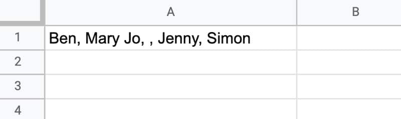
This simple SPLIT formula will separate these names, using the comma as the separator:

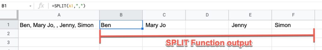
=SPLIT(A1,",")

The result is 5 cells, each containing a name. Note that one cell looks blank because the text string in cell A1 has two adjacent commas with a space between them. The “space” is interpreted in the same way as the names and contained in the output:

Split Function Name Example

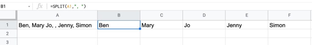
Now watch what happens if we include a space in the delimiter, i.e. ", "

=SPLIT(A1,", ")

The function splits on the comma "," and on the space " ", so the name “Mary Jo” split in two:

Undesirable behavior with SPLIT formula

This is probably not the desired behavior.

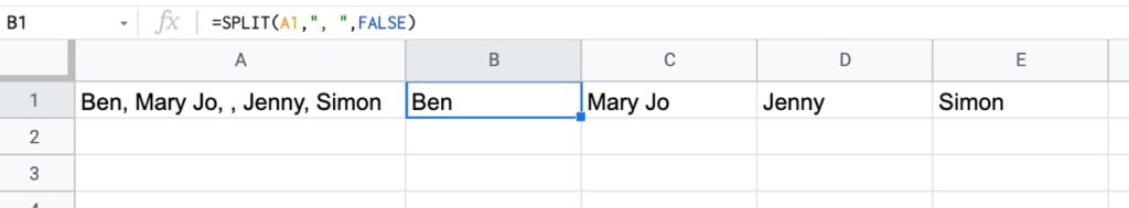
The third argument is an optional TRUE or FALSE that determines whether SPLIT considers each individual character of the delimiter (TRUE) or only the full combination as the separator to use (FALSE).

In our example, adding FALSE ensures that it only considers the combined comma/space string as the delimiter:

=SPLIT(A1,", ", FALSE)

And the output looks like this:

Split names in Google Sheets

There is a fourth argument too, which is optional and takes a TRUE/FALS value. It determines whether to remove blank cells or not in the output.

To illustrate this, consider this arrangement of data separated by semi-colons. Note the presence of two adjacent semi-colons with no data between them:

Split Formula Fourth Argument

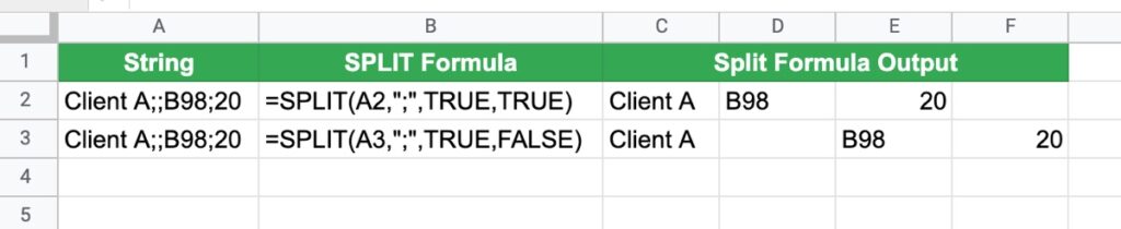
The fourth argument determines whether to show or hide the blank cell caused by the two adjacent semi-colons.

To keep the blank cells, add FALSE as the fourth argument:

=SPLIT(A2,",", TRUE, FALSE)

SPLIT Function in Google Sheets: Syntax

=SPLIT(text, delimiter, [split_by_each], [remove_empty_text])

It takes 4 arguments:

text

This is the text string or value in the cell that you want to split. It can also be a reference to a cell with a value in, or even the output of a nested formula, provided that output is a string or value and not an array.

delimiter

The character or characters used to split the text. Note that by default, all characters are used in the division. So a delimiter of “the” will split a text string on “the”, “he”,”t”,”h”,”e” etc.

This behavior can be controlled by the next argument:

split_by_each

This argument is optional and takes a TRUE or FALSE value only. If omitted, it’s assumed to be TRUE.

The TRUE behavior splits by individual characters in the delimiter and any combination of them. The FALSE behavior does not consider the characters separately, and only divides on the entire delimiter.

remove_empty_text

The fourth and final argument is optional and takes a TRUE or FALSE value only. If omitted, it’s assumed to be TRUE.

It specifies what to do with empty results in the SPLIT output. For example, suppose you’re splitting a text string with a "," and your string looks like this: “Ben,Bob,,Jenny,Anna”

Between the names Bob and Jenny are two commas with no value between them.

Setting this final argument of the SPLIT function to FALSE results in a blank cell in the output. If this fourth argument is omitted or set to TRUE, then the blank cell is removed and “Bob” and “Jenny” appear in adjacent cells.

SPLIT Function Notes

Delimiters in SPLIT are case sensitive. So “t” only splits on lower-case t’s in the text
The SPLIT function requires enough “space” for its output. If it splits a text string into 4 elements then it requires 4 cells (including the one the formula is in) on that row to expand into. If there is already data in any of these cells, it does NOT overwrite it but instead shows a #REF! error message
You can input a range as the first argument to the SPLIT function, but it requires an Array Formula wrapper to work
The output from the SPLIT function is an array of values that can be passed as the input into another formula, which may require the use of the Array Formula

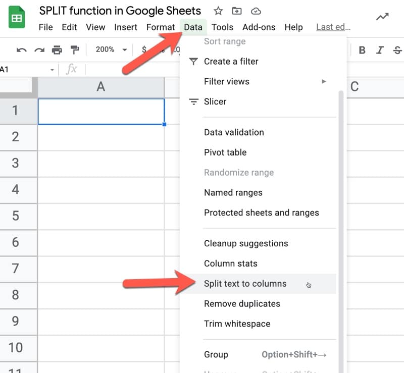
Alternative Split Method

There’s an alternative way to split values in a Google Sheet.

Under the Data menu, there’s a feature called “Split text to columns” which will separate single columns into multiple columns, based on the delimiter you specify.

It’s a quick and easy way to split text.

Note that it overwrites existing data in your Sheet if the split columns overlap with any existing data.

Split function alternative

SPLIT Function Template

Click here to open a view-only copy >>

Feel free to make a copy: File > Make a copy…

If you can’t access the template, it might be because of your organization’s Google Workspace settings. If you click the link and open it in an Incognito window you’ll be able to see it.

You can also read about it in the Google documentation.

Advanced Examples of the SPLIT Formula in Google Sheets

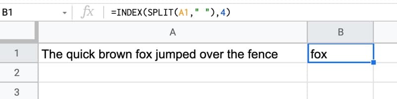
Extract The N-th Word In A Sentence

You can wrap the SPLIT function output with an INDEX function to extract the word at a given position in a sentence. E.g. to extract the 4th word, use this formula:

=INDEX(SPLIT(A1," "),4)

Extract Nth Word in Google Sheets

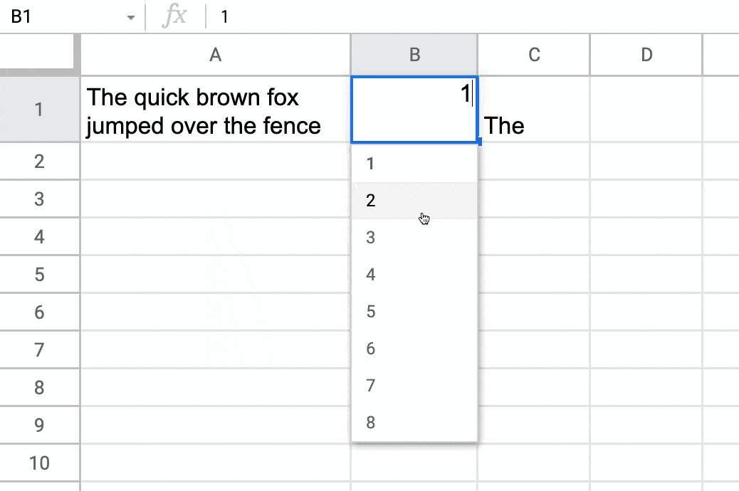
If you combine this with a drop down menu using data validation, you can create a word extractor:

extract Nth Word Data Validation

Alphabetize Comma-Separated Strings With The SPLIT Function in Google Sheets

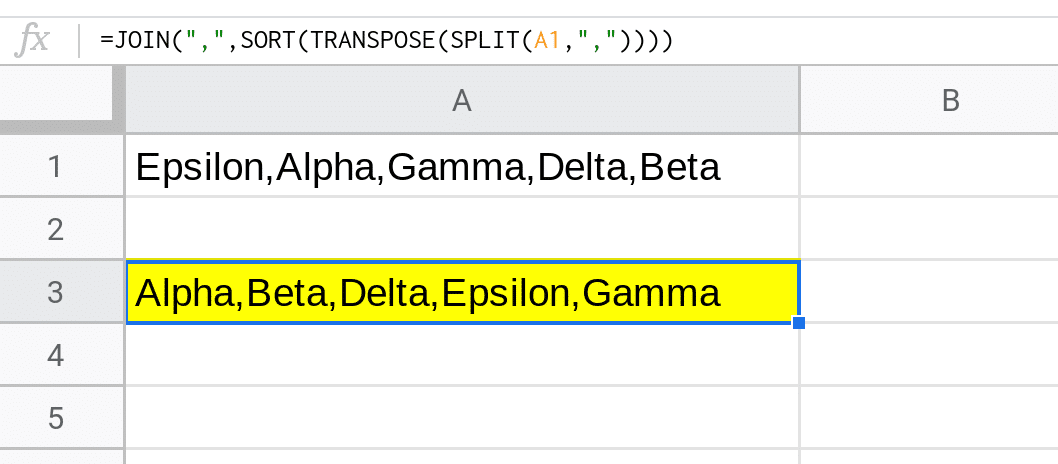
Suppose you have a list of words in a single cell that you want to sort alphabetically:

Formula Challenge 3

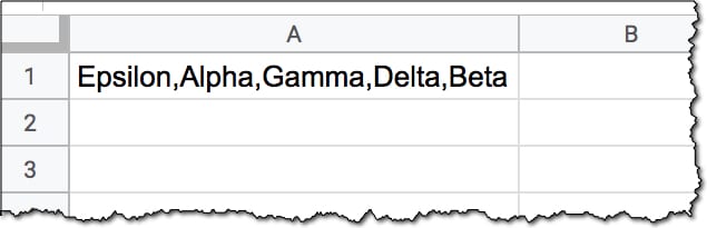
This formula will rearrange that list alphabetically:

=JOIN(",",SORT(TRANSPOSE(SPLIT(A1,","))))

It splits the string of words, applies the TRANSPOSE function to convert into a column so it can be sorted using the SORT function, and then recombines it with the JOIN function.

Formula Challenge 3 Solution

Splitting and Concatenating Strings

The SPLIT is useful in more advanced formulas as a way to divide an array into separate elements, do some work on those elements (e.g. sort them) before recombining them with another function, like the JOIN function.

For example, this array formula will add surnames to a list of first names in a cell:

=ArrayFormula(TRIM(JOIN(", ",SPLIT(A2,", ")&" Smith")))

which looks like this in your Google Sheet:

Split Function In Google Sheets To Add Surnames

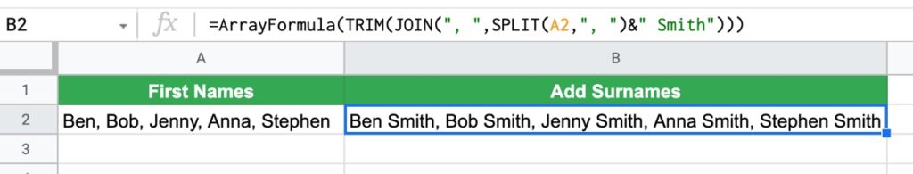
Using the onion framework to analyze this formula, starting from the innermost function and working out, it splits the text string, joins on the surname “Smith”, trims the excess trailing space with the TRIM function, and finally outputs an array by using the Array Formula.

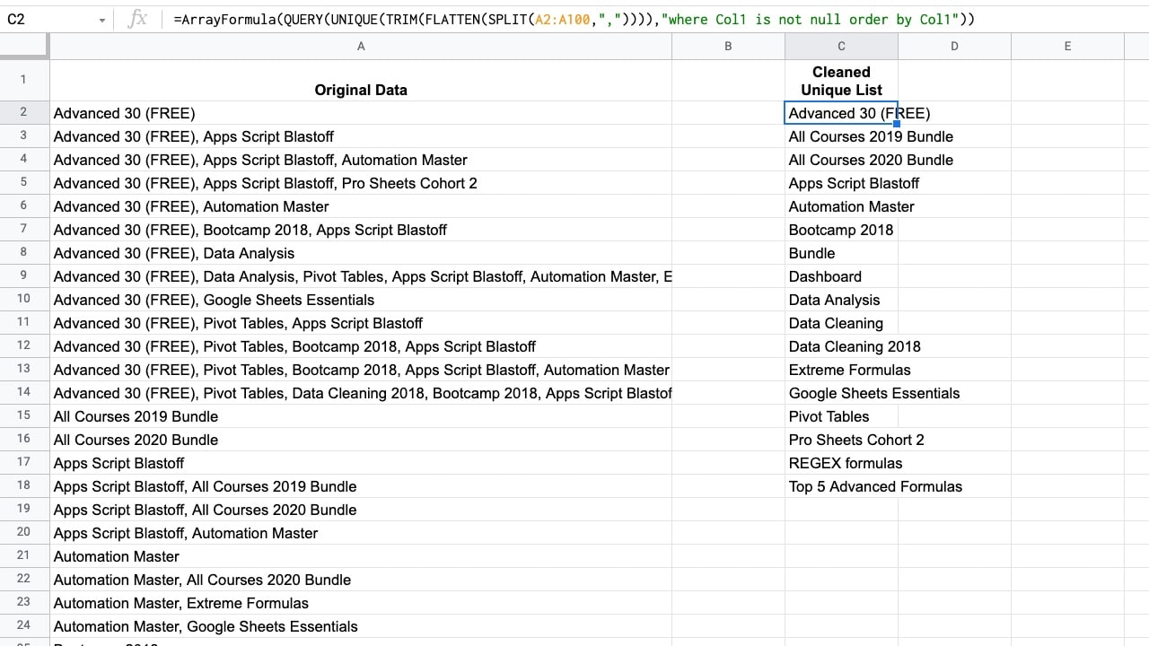
Find Unique Items In A Grouped List

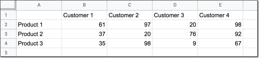
Suppose you want to find unique values from data that looks like this:

You want to extract a unique list of items from the column containing grouped words, which are separated by commas.

Use this formula to extract the unique values:

=ArrayFormula( QUERY( UNIQUE( TRIM( FLATTEN( SPLIT(A2:A100,",")))),"where Col1 is not null order by Col1"))

Read more about this technique in this post: Get A Unique List Of Items From A Column With Grouped Words

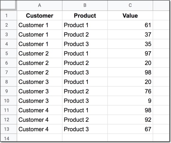
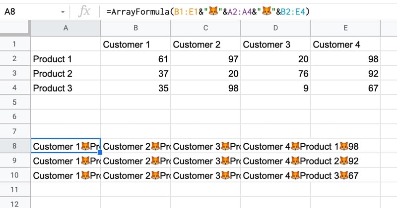
Unpivot Technique

The SPLIT function in Google Sheets is used in a number of the complex IMPORT formulas for retrieving social media statistics into your Google Sheet.

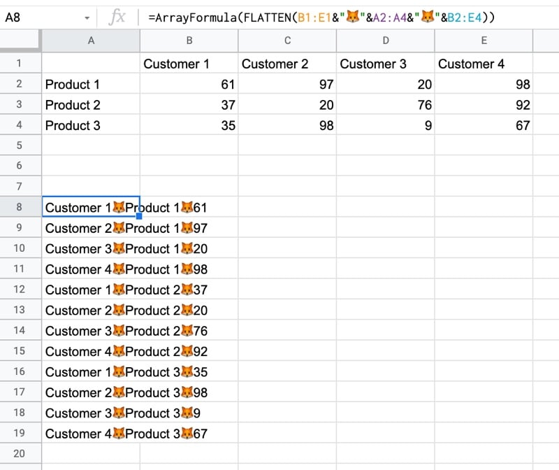
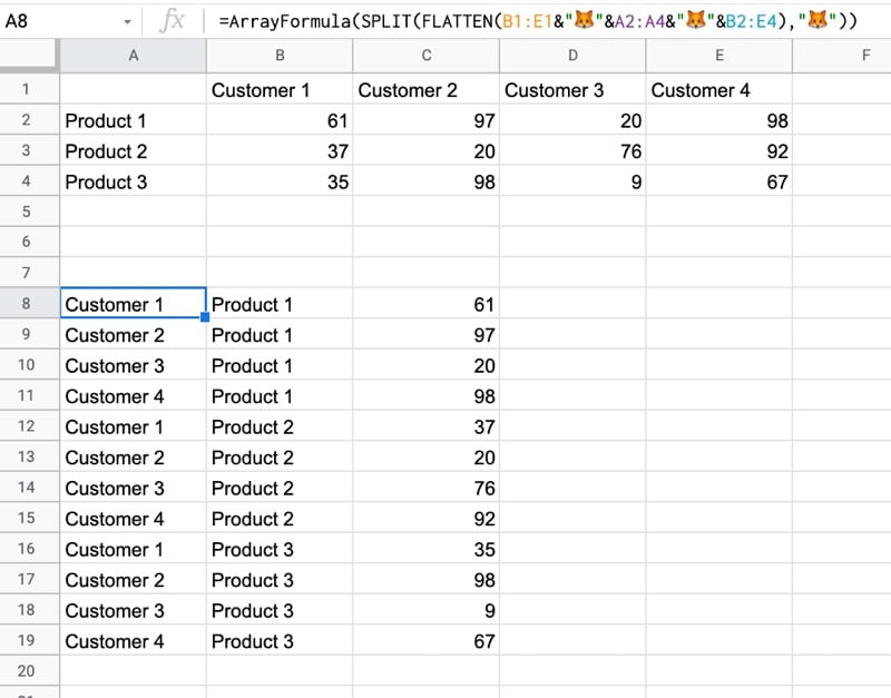
The SPLIT function was combined with the FLATTEN function in this exceedingly wacky unpivot formula in Google Sheets: