Let’s start with a mind-blowing fact, and then use the FACT function in Google Sheets to explain it.
Pick up a standard 52 card deck and give it a good shuffle.
The order of cards in a shuffled deck will be unique.
One that has likely never been seen before in the history of the universe and will likely never be seen again.
I’ll let that sink in.
Isn’t that mind-blowing?
Especially when you picture all the crazy casinos in Las Vegas.
Let’s understand why, and in the process learn about the FACT function and basic combinatorics (the study of counting in mathematics).
Four Card Deck
To keep things simple, suppose you only have 4 cards in your deck, the four aces.
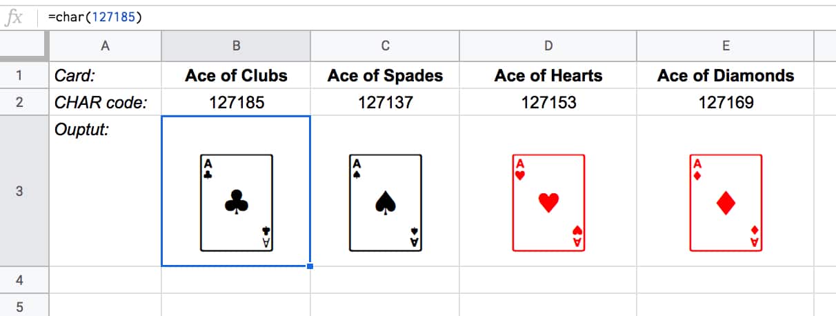
You can create this deck in Google Sheets with the CHAR function:
The formulas to create these four cards are:
Ace of Clubs:
=CHAR(127185)
Ace of Spades:
=CHAR(127137)
Ace of Hearts:
=CHAR(127153)
Ace of Diamonds:
=CHAR(127169)
Let’s see how many different combinations exist with just these four cards.
Pick one of them to start. You have a choice of four cards at this stage.
Once you’ve chosen the first one, you have three cards left, so there are 3 possible options for the second card choice.
When you’ve picked that second card, you have two cards left. So you have a choice of two for the third card.
The final card is the last remaining one.
So you have 4 choices * 3 choices * 2 choices * 1 choice = 4 * 3 * 2 * 1 = 24
There are 24 permutations (variations) with just 4 cards!
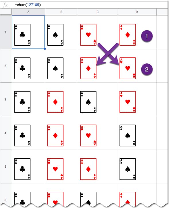
Visually, we can show this in our Google Sheet by displaying all the different combinations with the card images from above:
(I’ve just shown the first 6 rows for brevity.)
You can see for example, when moving from row 1 to row 2, we swapped the position of the two red suits: the Ace of Hearts and the Ace of Diamonds.
Five Card Deck
This time there are 5 choices for the first card, then 4, then 3, then 2, and finally 1.
So the number of permutations is 5 * 4 * 3 * 2 * 1 = 120
Already a lot more! I have not drawn this out in a Google Sheet and leave that as an optional exercise for you if you wish.
The FACT function
The FACT function in Google Sheets (see documentation) is a math function that returns the factorial of a given number. The factorial is the product of that number with all the numbers lower than it down to 1.
In other words, exactly what we’ve done above in the above calculations.
Four:
The 4 card deck formula is:
=FACT(4)
which gives an answer of 24 permutations.
Five:
The 5 card deck formula is:
=FACT(5)
which gives an answer of 120 permutations.
Six:
A 6 card deck is:
=FACT(6)
which gives an answer of 720 permutations.
Twelve:
A 12 card deck has 479,001,600 different ways of being shuffled:
=FACT(12)
(You’re more likely to win the Powerball lottery at 1 in 292 million odds than to get two matching shuffled decks of cards, even with just 12 cards!)
Fifty Two:
Keep going up to a full deck of 52 cards with the formula and it’s a staggeringly large number.
=FACT(52)
Type it into Google Sheets and you’ll see an answer of 8.07E+67, which is 8 followed by 67 zeros!
(This number notation is called scientific notation, where huge numbers are rounded to the first few digits multiplied by a 10 to the power of some number, 67 in this case.)
This answer is more than the number of stars in the universe (about 10 followed by 21 zeros).
Put another way if all 6 billion humans on earth began shuffling cards at 1 deck per minute every day of the year for millions of years, we still wouldn’t even be close to finding all possible combinations.
Unpivot in Google Sheets is a method to turn “wide” tables into “tall” tables, which are more convenient for analysis.
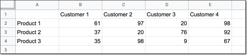
Suppose we have a wide table like this:
Wide data like this is good for the Google Sheets chart tool but it’s not ideal for creating pivot tables or doing analysis. The main reason is that data is captured in the column headings, which prevents you using it in pivot tables for analyis.
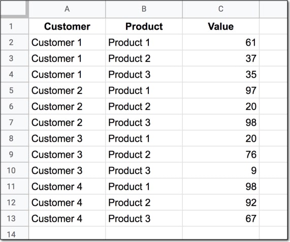
So we want to transform this data — unpivot it — into the tall format that is the way databases store data:
But how do we unpivot our data like that?
It turns out it’s quite hard.
It’s harder than going the other direction, turning tall data into wide data tables, which we can do with a pivot table.
This article looks at how to do it using formulas so if you’re ready for some complex formulas, let’s dive in…
Unpivot in Google Sheets
We’ll use the wide dataset shown in the first image at the top of this post.
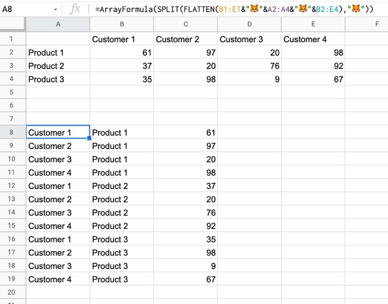
The output of our formulas should look like the second image in this post.
In other words, we need to create 16 rows to account for the different pairings of Customer and Product, e.g. Customer 1 + Product 1, Customer 1 + Product 2, etc. all the way up to Customer 4 + Product 4.
Of course, we’ll employ the Onion Method to understand these formulas.
Feel free to make your own copy (File > Make a copy…).
(If you can’t open the file, it’s likely because your G Suite account prohibits opening files from external sources. Talk to your G Suite administrator or try opening the file in an incognito browser.)
Step 1: Combine The Data
Use an array formula like this to combine the column headings (Customer 1, Customer 2, etc.) with the row headings (Product 1, Product 2, Product 3, etc.) and the data.
It’s crucial to add a special character between these sections of the dataset though, so we can split them up later on. I’ve used the fox emoji (because, why not?) but you can use whatever you like, provided it’s unique and doesn’t occur anywhere in the dataset.
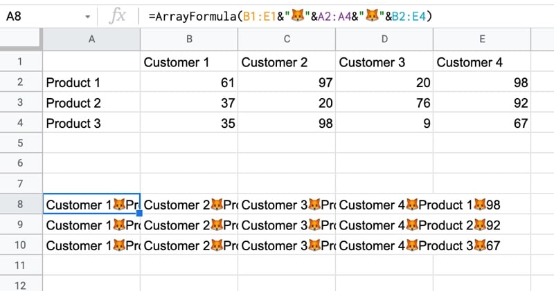
=ArrayFormula(B1:E1&"🦊"&A2:A4&"🦊"&B2:E4)
The output of this formula is:
Step 2: Flatten The Data
Before the introduction of the FLATTEN function, this step was much, much harder, involving lots of weird formulas.
Thankfully the FLATTEN function does away with all of that and simply stacks all of the columns in the range on top of each other. So in this example, our combined data turns into a single column.
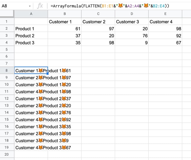
=ArrayFormula(FLATTEN(B1:E1&"🦊"&A2:A4&"🦊"&B2:E4))
The result is:
Step 3: Split The Data Into Columns
The final step is to split this new tall column into separate columns for each data type. You can see now why we needed to include the fox emoji so that we have a unique character to split the data on.
Wrap the formula from step 2 with the SPLIT function and set the delimiter to “🦊”:
Google Apps Script is a cloud-based scripting language for extending the functionality of Google Apps and building lightweight cloud-based applications.
It means you write small programs with Apps Script to extend the standard features of Google Workspace Apps. It’s great for filling in the gaps in your workflows.
With Apps Script, you can do cool stuff like automating repeatable tasks, creating documents, emailing people automatically and connecting your Google Sheets to other services you use.
Writing your first Google Script
In this Google Sheets script tutorial, we’re going to write a script that is bound to our Google Sheet. This is called a container-bound script.
(If you’re looking for more advanced examples and tutorials, check out the full list of Apps Script articles on my homepage.)
Hello World in Google Apps Script
Let’s write our first, extremely basic program, the classic “Hello world” program beloved of computer teaching departments the world over.
Begin by creating a new Google Sheet.
Then click the menu: Extensions > Apps Script
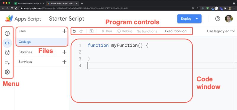
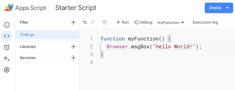
This will open a new tab in your browser, which is the Google Apps Script editor window:
By default, it’ll open with a single Google Script file (code.gs) and a default code block, myFunction():
function myFunction() {

}
In the code window, between the curly braces after the function myFunction() syntax, write the following line of code so you have this in your code window:
function myFunction() {
  Browser.msgBox("Hello World!");
}
Your code window should now look like this:
Google Apps Script Authorization
Google Scripts have robust security protections to reduce risk from unverified apps, so we go through the authorization workflow when we first authorize our own apps.
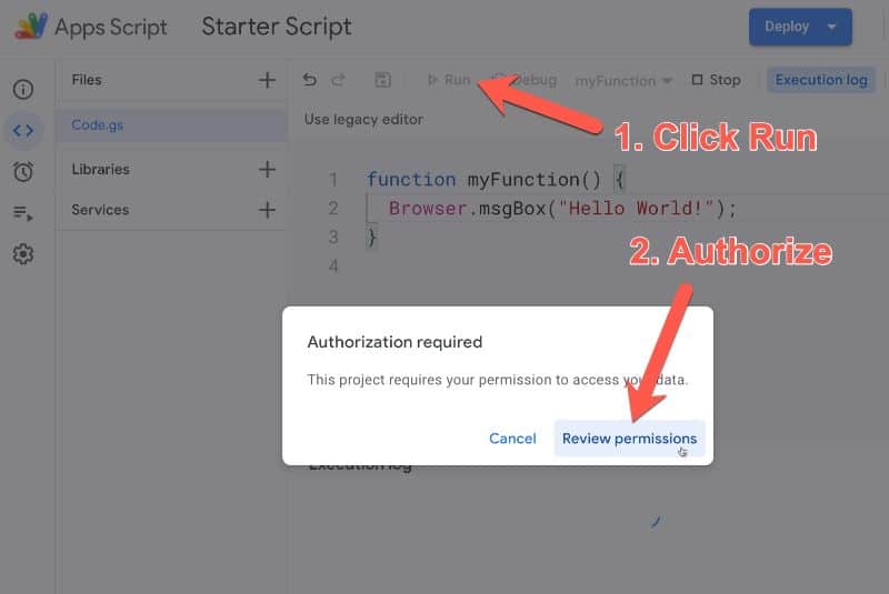
When you hit the run button for the first time, you will be prompted to authorize the app to run:
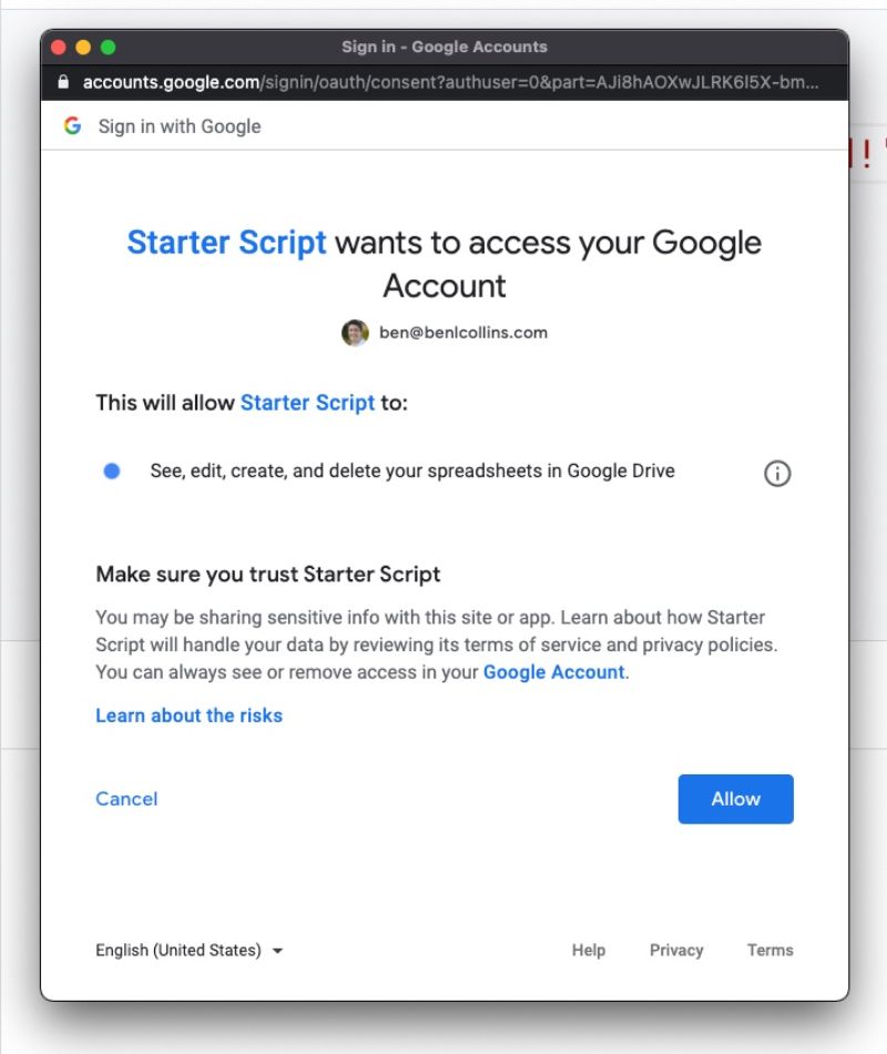
Clicking Review Permissions pops up another window in turn, showing what permissions your app needs to run. In this instance the app wants to view and manage your spreadsheets in Google Drive, so click Allow (otherwise your script won’t be able to interact with your spreadsheet or do anything):
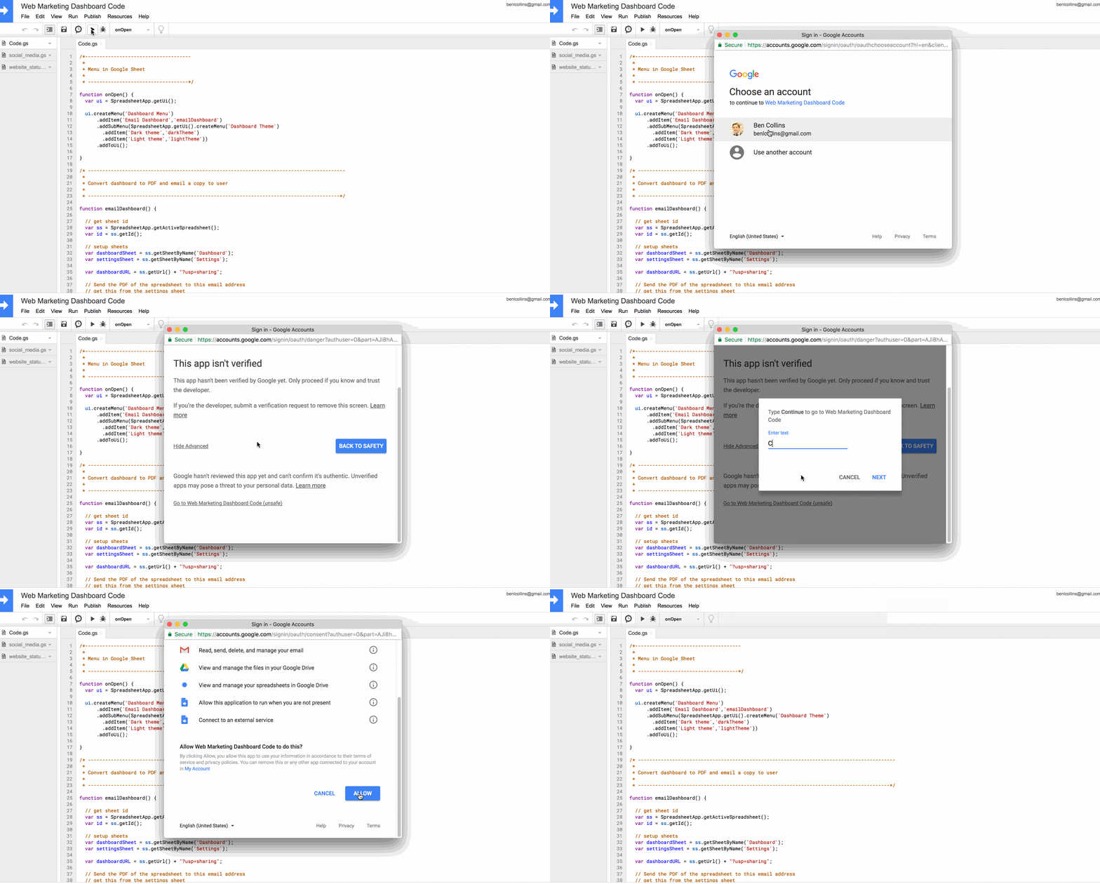
❗️When your first run your apps script, you may see the “app isn’t verified” screen and warnings about whether you want to continue.
In our case, since we are the creator of the app, we know it’s safe so we do want to continue. Furthermore, the apps script projects in this post are not intended to be published publicly for other users, so we don’t need to submit it to Google for review (although if you want to do that, here’s more information).
Click the “Advanced” button in the bottom left of the review permissions pop-up, and then click the “Go to Starter Script Code (unsafe)” at the bottom of the next screen to continue. Then type in the words “Continue” on the next screen, click Next, and finally review the permissions and click “ALLOW”, as shown in this image (showing a different script in the old editor):
Once you’ve authorized the Google App script, the function will run (or execute).
If anything goes wrong with your code, this is the stage when you’d see a warning message (instead of the yellow message, you’ll get a red box with an error message in it).
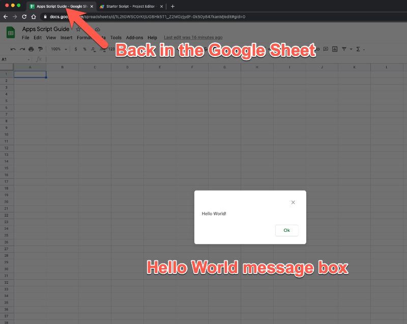
Return to your Google Sheet and you should see the output of your program, a message box popup with the classic “Hello world!” message:
Click on Ok to dismiss.
Great job! You’ve now written your first apps script program.
Rename functions in Google Apps Script
We should rename our function to something more meaningful.
At present, it’s called myFunction which is the default, generic name generated by Google. Every time I want to call this function (i.e. run it to do something) I would write myFunction(). This isn’t very descriptive, so let’s rename it to helloWorld(), which gives us some context.
So change your code in line 1 from this:
function myFunction() {
  Browser.msgBox("Hello World!");
}
to this:
function helloWorld() {
  Browser.msgBox("Hello World!");
}
Note, it’s convention in Apps Script to use the CamelCase naming convention, starting with a lowercase letter. Hence, we name our function helloWorld, with a lowercase h at the start of hello and an uppercase W at the start of World.
Adding a custom menu in Google Apps Script
In its current form, our program is pretty useless for many reasons, not least because we can only run it from the script editor window and not from our spreadsheet.
Let’s fix that by adding a custom menu to the menu bar of our spreadsheet so a user can run the script within the spreadsheet without needing to open up the editor window.
This is actually surprisingly easy to do, requiring only a few lines of code. Add the following 6 lines of code into the editor window, above the helloWorld() function we created above, as shown here:
If you look back at your spreadsheet tab in the browser now, nothing will have changed. You won’t have the custom menu there yet. We need to re-open our spreadsheet (refresh it) or run our onOpen() script first, for the menu to show up.
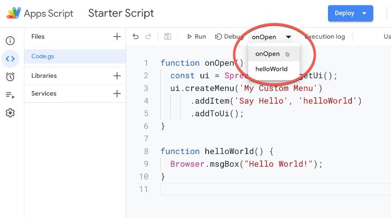
To run onOpen() from the editor window, first select then run the onOpen function as shown in this image:
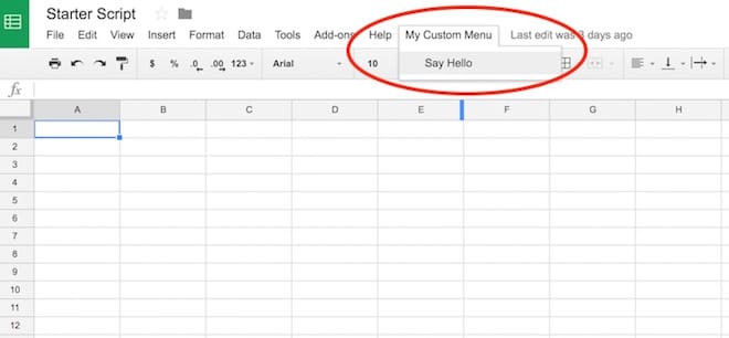
Now, when you return to your spreadsheet you’ll see a new menu on the right side of the Help option, called My Custom Menu. Click on it and it’ll open up to show a choice to run your Hello World program:
Run functions from buttons in Google Sheets
An alternative way to run Google Scripts from your Sheets is to bind the function to a button in your Sheet.
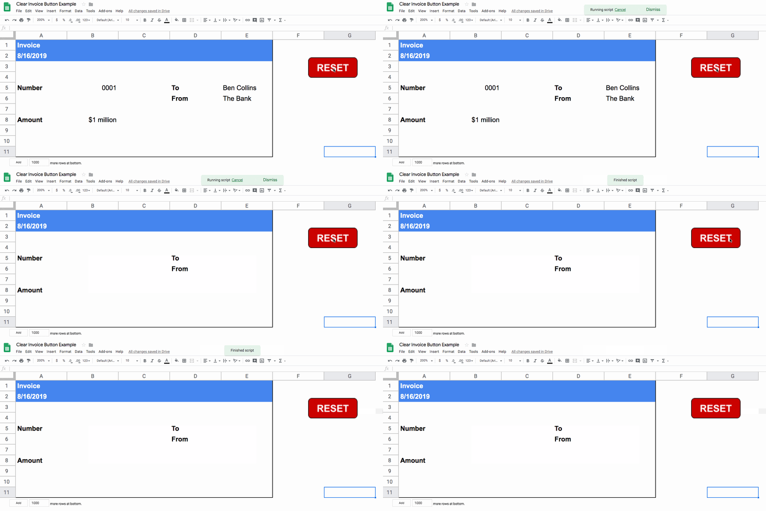
For example, here’s an invoice template Sheet with a RESET button to clear out the contents:
Another great way to get started with Google Scripts is by using Macros. Macros are small programs in your Google Sheets that you record so that you can re-use them (for example applying standard formatting to a table). They use Apps Script under the hood so it’s a great way to get started.
Let’s create a custom function with Apps Script, and also demonstrate the use of the Maps Service. We’ll be creating a small custom function that calculates the driving distance between two points, based on Google Maps Service driving estimates.
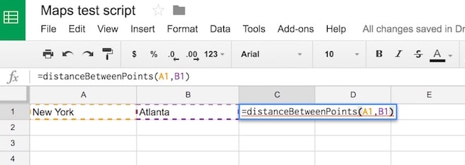
The goal is to be able to have two place-names in our spreadsheet, and type the new function in a new cell to get the distance, as follows:
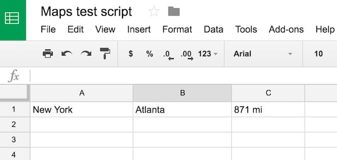
The solution should be:
Copy the following code into the Apps Script editor window and save. First time, you’ll need to run the script once from the editor window and click “Allow” to ensure the script can interact with your spreadsheet.
function distanceBetweenPoints(start_point, end_point) {
  // get the directions
  const directions = Maps.newDirectionFinder()
     .setOrigin(start_point)
     .setDestination(end_point)
     .setMode(Maps.DirectionFinder.Mode.DRIVING)
     .getDirections();

  // get the first route and return the distance
  const route = directions.routes[0];
  const distance = route.legs[0].distance.text;
  return distance;
}
Saving data with Google Apps Script
Let’s take a look at another simple use case for this Google Sheets Apps Script tutorial.
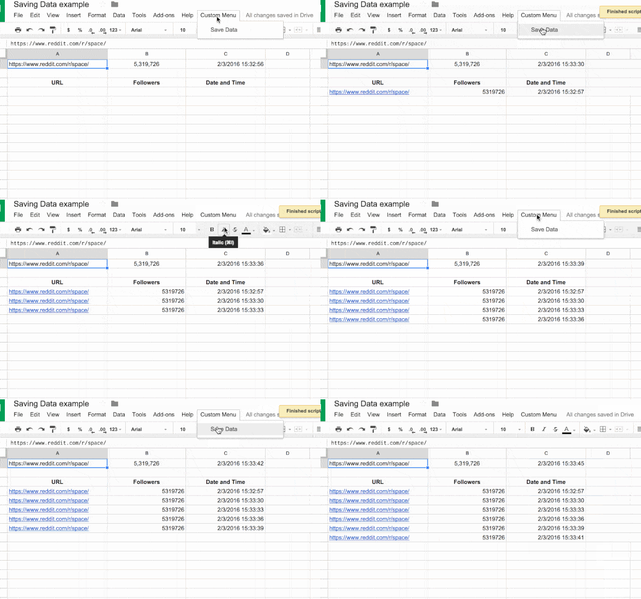
Suppose I want to save copy of some data at periodic intervals, like so:
In this script, I’ve created a custom menu to run my main function. The main function, saveData(), copies the top row of my spreadsheet (the live data) and pastes it to the next blank line below my current data range with the new timestamp, thereby “saving” a snapshot in time.
The code for this example is:
// custom menu function
function onOpen() {
  const ui = SpreadsheetApp.getUi();
  ui.createMenu('Custom Menu')
      .addItem('Save Data','saveData')
      .addToUi();
}

// function to save data
function saveData() {
  const ss = SpreadsheetApp.getActiveSpreadsheet();
  const sheet = ss.getSheets()[0];
  const url = sheet.getRange('Sheet1!A1').getValue();
  const follower_count = sheet.getRange('Sheet1!B1').getValue();
  const date = sheet.getRange('Sheet1!C1').getValue();
  sheet.appendRow([url,follower_count,date]);
}
2. Open script editor from the menu: Extensions > Apps Script
3. In the newly opened Script tab, remove all of the boilerplate code (the “myFunction” code block)
4. Copy in the following code:
// code to add the custom menu
function onOpen() {
  const ui = DocumentApp.getUi();
  ui.createMenu('My Custom Menu')
      .addItem('Insert Symbol', 'insertSymbol')
      .addToUi();
}

// code to insert the symbol
function insertSymbol() {
  // add symbol at the cursor position
  const cursor = DocumentApp.getActiveDocument().getCursor();
  cursor.insertText('§§');

}
5. You can change the special character in this line
cursor.insertText('§§');
to whatever you want it to be, e.g.
cursor.insertText('( ͡° ͜ʖ ͡°)');
6. Click Save and give your script project a name (doesn’t affect the running so call it what you want e.g. Insert Symbol)
7. Run the script for the first time by clicking on the menu: Run > onOpen
8. Google will recognize the script is not yet authorized and ask you if you want to continue. Click Continue
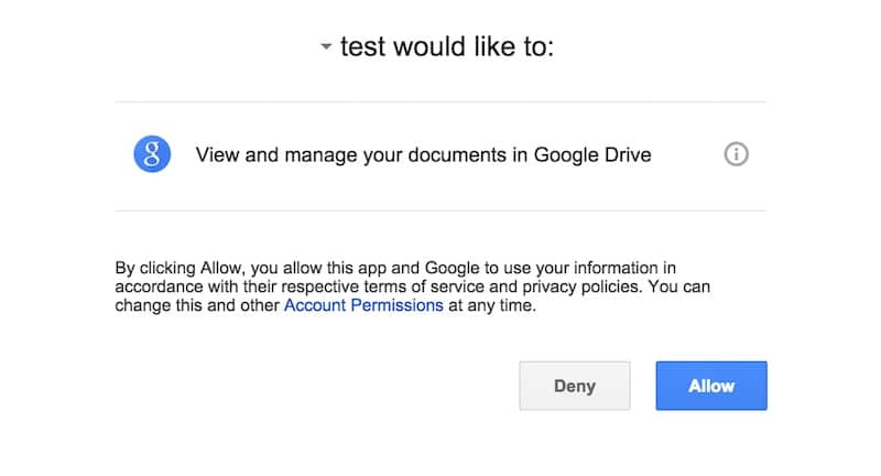
9. Since this the first run of the script, Google Docs asks you to authorize the script (I called my script “test” which you can see below):
10. Click Allow
11. Return to your Google Doc now.
12. You’ll have a new menu option, so click on it:
My Custom Menu > Insert Symbol
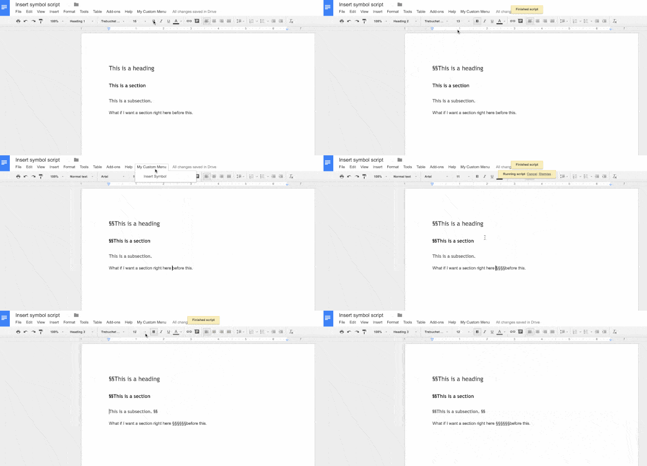
13. Click on Insert Symbol and you should see the symbol inserted wherever your cursor is.
Google Apps Script Tip: Use the Logger class
Use the Logger class to output text messages to the log files, to help debug code.
The log files are shown automatically after the program has finished running, or by going to the Executions menu in the left sidebar menu options (the fourth symbol, under the clock symbol).
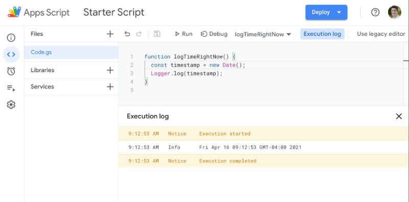
The syntax in its most basic form is Logger.log(something in here). This records the value(s) of variable(s) at different steps of your program.
For example, add this script to a code file your editor window:
function logTimeRightNow() {
  const timestamp = new Date();
  Logger.log(timestamp);
}
Run the script in the editor window and you should see:
Real world examples from my own work
I’ve only scratched the surface of what’s possible using G.A.S. to extend the Google Apps experience.
Here are a couple of interesting projects I’ve worked on:
1) A Sheets/web-app consisting of a custom web form that feeds data into a Google Sheet (including uploading images to Drive and showing thumbnails in the spreadsheet), then creates a PDF copy of the data in the spreadsheet and automatically emails it to the users. And with all the data in a master Google Sheet, it’s possible to perform data analysis, build dashboards showing data in real-time and share/collaborate with other users.
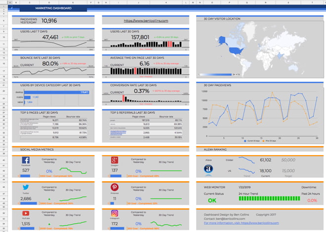
2) A dashboard that connects to a Google Analytics account, pulls in social media data, checks the website status and emails a summary screenshot as a PDF at the end of each day.
Imagination and patience to learn are the only limits to what you can do and where you can go with GAS. I hope you feel inspired to try extending your Sheets and Docs and automate those boring, repetitive tasks!
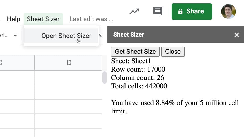
In this tutorial, you’ll use Apps Script to build a tool called Sheet Sizer, to measure the size of your Google Sheets!
Google Sheets has a limit of 10 million cells, but it’s hard to know how much of this space you’ve used.
Sheet Sizer will calculate the size of your Sheet and compare it to the 10 million cell limit in Google Sheets.
Sheet Sizer: Build a sidebar to display information
Step 1:
Open a blank sheet and rename it to “Sheet Sizer”
Step 2:
Open the IDE. Go to Tools > Script editor
Step 3:
Rename your script file “Sheet Sizer Code”
Step 4:
In the Code.gs file, delete the existing “myFunction” code and copy in this code:
/**
* Add custom menu to sheet
*/
function onOpen() {

  SpreadsheetApp.getUi()
    .createMenu('Sheet Sizer')
    .addItem('Open Sheet Sizer', 'showSidebar')
    .addToUi();
}

/**
* function to show sidebar
*/
function showSidebar() {

  // create sidebar with HTML Service
  const html = HtmlService.createHtmlOutputFromFile('Sidebar').setTitle('Sheet Sizer');

// add sidebar to spreadsheet UI
  SpreadsheetApp.getUi().showSidebar(html);
}
There are two functions: onOpen, which will add the custom menu to your Sheet, and showSidebar, which will open a sidebar.
The text between the /* ... */ or lines starting with // are comments.
Step 5:
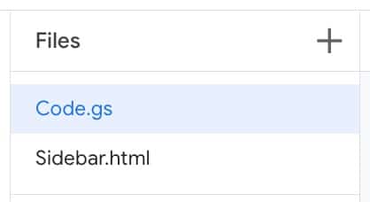
Click the + next to Files in the left menu, just above the Code.gs filename.
Add an HTML file and call it “Sidebar”. It should look like this:
Step 6:
In the Sidebar file, on line 7, between the two BODY tags of the existing code, copy in the following code:
Step 8:
Select the Code.gs file, then select the onOpen function in the menu bar (from the drop down next to the word Debug). Then hit Run.
Step 9:
When you run for the first time, you have to accept the script permissions. If you see an “App isn’t verified” screen, click on Advanced, then “Go to…” and follow the prompts. (More info here.)
Step 10:
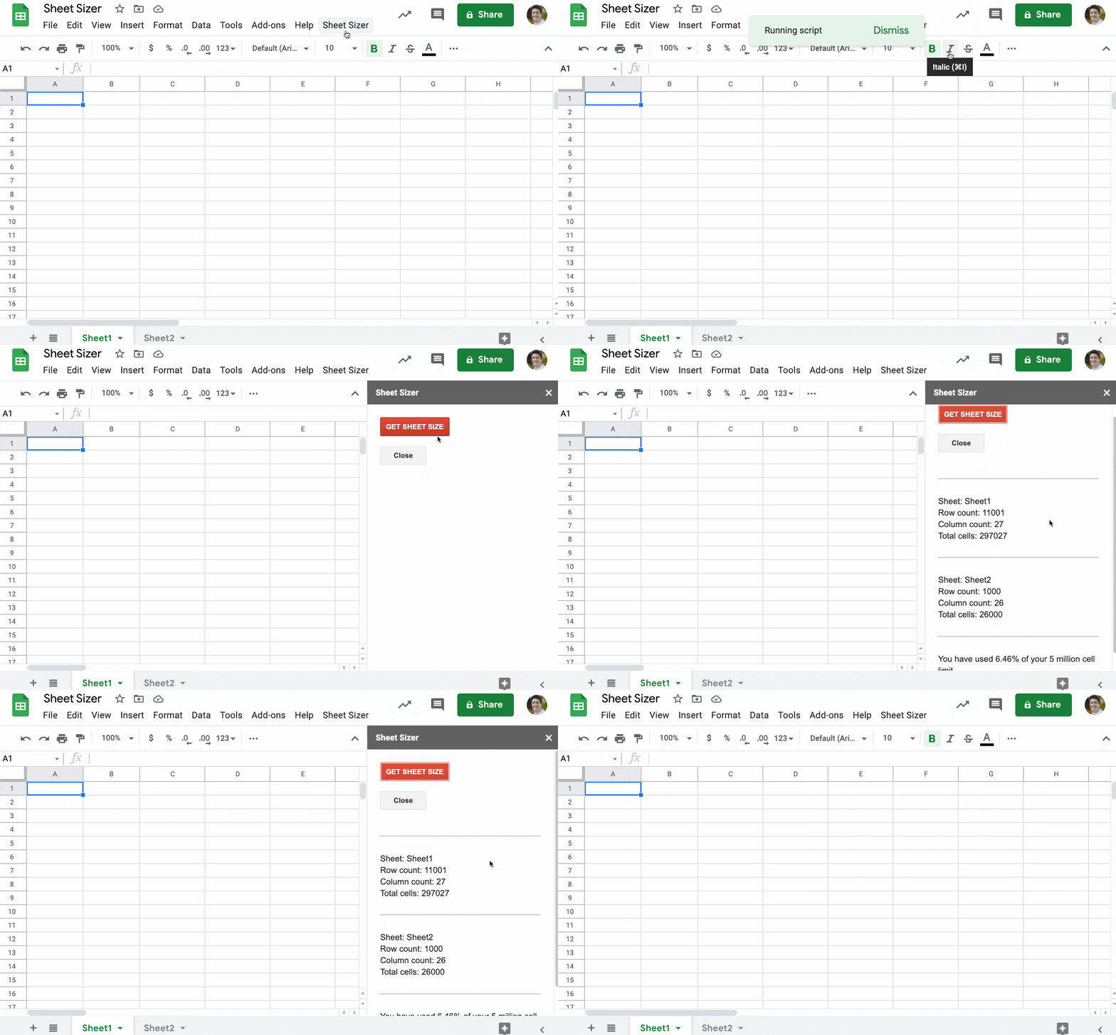
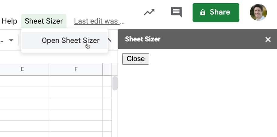
After authorizing the app in step 8, jump back to your Google Sheet. You should see a new custom menu “Sheet Sizer” in the menu bar, to the right of the Help menu.
Click the menu to open the sidebar.
Step 11:
Close the menu using the button.
Here’s what you’ve built so far:
Sheet Sizer: Add a new button and functionality to the sidebar
Step 12:
In the Sidebar file, after the first BODY tag, on line 6, and before the INPUT tag on line 7, add a new line.
When clicked, this will run a function called getSheetSize.
Step 13:
Add the getSheetSize function into the Sidebar file with the following code.
Copy and paste this after the two INPUT tags but before the final BODY tag, on line 9.
<script>
function getSheetSize() {

  google.script.run.auditSheet();

}
</script>
When the button is clicked to run the getSheetSize function (client side, in the sidebar), it will now run a function called auditSheet in our Apps Script (server side).
Step 14:
Go to the Code.gs file
Step 15:
Copy and paste this new function underneath the rest of your code:
/**
* Get size data for a given sheet url
*/
function auditSheet() {
  // get Sheet
  const ss = SpreadsheetApp.getActiveSpreadsheet();
  const sheet = ss.getActiveSheet();

  // get sheet name
  const name = sheet.getName();

  // get current sheet dimensions
  const maxRows = sheet.getMaxRows();
  const maxCols = sheet.getMaxColumns();
  const totalCells = maxRows * maxCols;

  // output
  SpreadsheetApp.getUi().alert(totalCells);
}
This gets the active Sheet of your spreadsheet and calculates the total number of cells as max rows multiplied by max columns.
Finally, the last line displays an alert popup to show the total number.
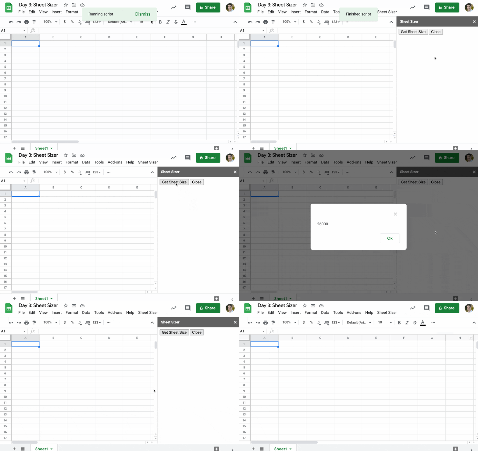
Step 16:
Back in your Google Sheet, run Sheet Sizer from the custom Sheet Sizer menu.
When you click on the “Get Sheet Size” button, you should see a popup that shows the number of cells in your Sheet:
Sheet Sizer: Display the Sheet size in the sidebar
Step 17:
Delete this line of code in the auditSheet function:
SpreadsheetApp.getUi().alert(totalCells);
Step 18:
Paste in this new code, to replace the code you deleted in Step 4:
// put variables into object
const sheetSize = 'Sheet: ' + name +
  '<br>Row count: ' + maxRows +
  '<br>Column count: ' + maxCols +
  '<br>Total cells: ' + totalCells +
  '<br><br>You have used ' + ((totalCells / 5000000)*100).toFixed(2) + '% of your 10 million cell limit.';

return sheetSize;
Now, instead of showing the total number of cells in an alert popup, it sends the result back to the sidebar.
Let’s see how to display this result in your sidebar.
Step 19:
Go to the Sidebar file and copy this code after the two INPUT tags but before the first SCRIPT tag:
<div id="results"></div>
This is a DIV tag that we’ll use to display the output.
Step 20:
Staying in the Sidebar file, replace this line of code:
It runs when the Apps Script function auditSheet successfully executes on the server side. The return value of that auditSheet function is passed to a new function called displayResults, which we’ll create now.
Step 21:
Underneath the getSheetSize function, add this function:
function displayResults(results) {
  // display results in sidebar
  document.getElementById("results").innerHTML = results;
}
When this function runs, it adds the results value (our total cells count) to that DIV tag of the sidebar you added in step 7.
Step 22:
Back in your Google Sheet, run Sheet Sizer from the custom Sheet Sizer menu.
When you click on the “Get Sheet Size” button, you should see a popup that shows the number of cells in your Sheet:
Sheet Sizer: Handle multiple sheets
Step 23:
Modify your auditSheet code to this:
/**
* Get size data for a given sheet url
*/
function auditSheet(sheet) {

  // get spreadsheet object
  const ss = SpreadsheetApp.getActiveSpreadsheet();

  // get sheet name
  const name = sheet.getName();

  // get current sheet dimensions
  const maxRows = sheet.getMaxRows();
  const maxCols = sheet.getMaxColumns();
  const totalCells = maxRows * maxCols;

  // put variables into object
  const sheetSize = {
    name: name,
    rows: maxRows,
    cols: maxCols,
    total: totalCells
  }

  // return object to function that called it
  return sheetSize;

}
Step 24:
In your Code.gs file, copy and paste the following code underneath the existing code:
/**
* Audits all Sheets and passes full data back to sidebar
*/
function auditAllSheets() {

  // get spreadsheet object
  const ss = SpreadsheetApp.getActiveSpreadsheet();
  const sheets = ss.getSheets();

  // declare variables
  let output = '';
  let grandTotal = 0;

  // loop over sheets and get data for each
  sheets.forEach(sheet => {

    // get sheet results for the sheet
    const results = auditSheet(sheet);

    // create output string from results
    output = output + '<br><hr><br>Sheet: ' + results.name +
      '<br>Row count: ' + results.rows +
      '<br>Column count: ' + results.cols +
      '<br>Total cells: ' + results.total + '<br>';

    // add results to grand total
    grandTotal = grandTotal + results.total;

  });

  // add grand total calculation to the output string
  output = output + '<br><hr><br>' +
    'You have used ' + ((grandTotal / 5000000)*100).toFixed(2) + '% of your 10 million cell limit.';

  // pass results back to sidebar
  return output;

}
This adds a new function, auditAllSheets, which loops over all the sheets in your Google Sheet and calls the auditSheet function for each one. The results for each Sheet are joined together into a result string, called output.
The callback function is the general auditAllSheets function, not the specific individual sheet function.
Step 26:
Back in your Google Sheet, add another sheet to your Google Sheet (if you haven’t already) and run Sheet Sizer.
It will now display the results for all the sheets within your Google Sheet!
Sheet Sizer: Add CSS styles
This step is purely cosmetic to make the sidebar more aesthetically pleasing.
Step 27:
Add these CSS lines inside the HEAD tags of the sidebar file:
<!-- Add CSS code to format the sidebar from google stylesheet -->
<link rel="stylesheet" href="https://ssl.gstatic.com/docs/script/css/add-ons1.css">

<style>
  body {
    padding: 20px;
  }
</style>
One final improvement from me is to move the 10 million cell limit number into a global variable.
Currently, it’s buried in your script so it’s difficult to find and update if and when Google updates the Sheets cell limit.
It’s not good practice to hard-code variables in your code for this reason.
The solution is to move it into a global variable at the top of your Code.gs file, with the following code:
/**
 * Global Variable
 */
const MAX_SHEET_CELLS = 10000000;
And then change the output line by replacing the 5000000 number with the new global variable MAX_SHEET_CELLS:
// add grand total calculation to the output string
output = output + '<br><hr><br>' +
  'You have used ' + ((grandTotal / MAX_SHEET_CELLS)*100).toFixed(2) + '% of your 10 million cell limit.';
Here is your final Sheet Sizer tool in action:
Click here to see the full code for the Sheet Sizer tool on GitHub.
Next steps: have a go at formatting the numbers shown in the sidebar, by adding thousand separators so that 1000 shows as 1,000 for example.
The Challenge: Merge Columns With Single Range Reference
Question: How can you merge n number of columns and get the unique values, without typing each one out?
In other words, can you create a single formula that gives the same output as this one:
=SORT( UNIQUE( {A:A;B:B;C:C;...;XX:XX} ))
but without having to write out A:A, B:B, C:C, D:D etc. and instead just write A:XX as in the input?
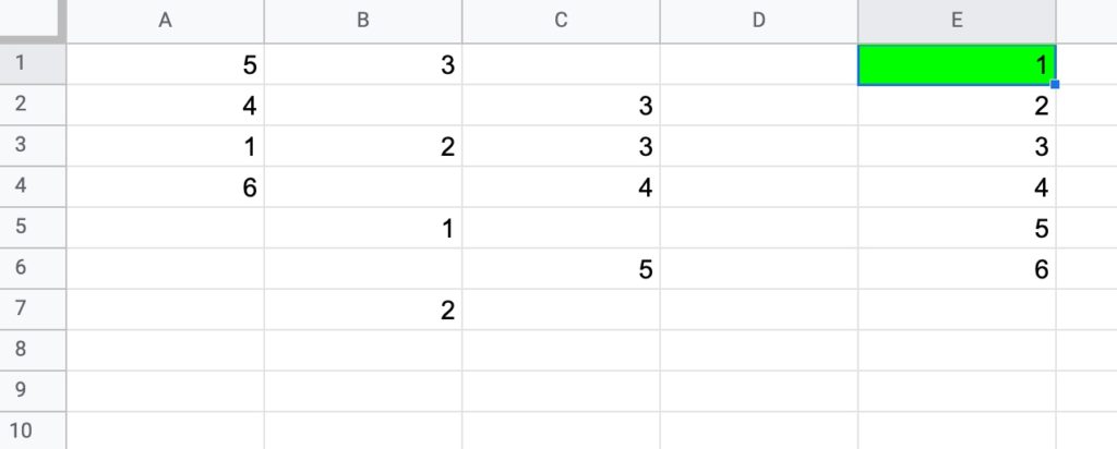
Use this simple dataset example, where your formula will be in cell E1 (in green):
Your answer should:
be a formula in a single cell
work with the input range in the form A:XX (e.g. A:C in this example)
work with numbers and/or text values
return only the unique values, in an ascending order in a SINGLE COLUMN.
Solutions To Sort A Column By Last Name
I received 67 replies to this formula challenge with two different methods for solving it. Congratulations to everyone who took part!
I learnt so much from the different replies, many of which proffered a shorter and more elegant second solution than my own original formula.
Here I present the two solutions.
There’s a lot to learn by looking through them.
1. FLATTEN method
=SORT(UNIQUE(FLATTEN(A:C)))
The formula uses the FLATTEN function to collect data from the input ranges into a single column before the UNIQUE function selects the unique ones before they are finally sorted.
Note 1: you can have multiple inputs (arguments) to the FLATTEN function. Data is ordered by the order of the inputs, then row and then column.
Note 2: at the moment the FLATTEN function doesn’t show up in the auto-complete when you start typing it out. You can still use it, but you’ll have to type it out fully yourself.
Thanks to the handful of you that shared this neat solution with me. Great work!
2. TEXTJOIN method
Join all the values in A:C with TEXTJOIN, using a unique character as the delimiter (in this case, the King and Queen chess pieces!)
You want to use an identifier that is not in columns A to C.
=TEXTJOIN("♔♕",TRUE,A:C)
Split on this unique delimiter using the SPLIT function:
=SPLIT(TEXTJOIN("♔♕",TRUE,A:C),"♔♕")
Use the TRANSPOSE function to switch to a column, select the unique values only and finally wrap with a sort function to get the result: