Unpivot in Google Sheets is a method to turn “wide” tables into “tall” tables, which are more convenient for analysis.
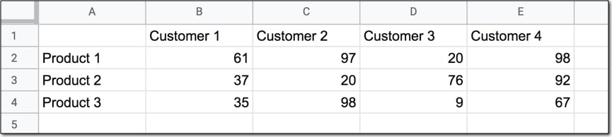
Suppose we have a wide table like this:
Wide data like this is good for the Google Sheets chart tool but it’s not ideal for creating pivot tables or doing analysis. The main reason is that data is captured in the column headings, which prevents you using it in pivot tables for analyis.
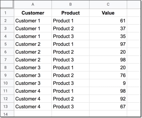
So we want to transform this data — unpivot it — into the tall format that is the way databases store data:
But how do we unpivot our data like that?
It turns out it’s quite hard.
It’s harder than going the other direction, turning tall data into wide data tables, which we can do with a pivot table.
This article looks at how to do it using formulas so if you’re ready for some complex formulas, let’s dive in…
Unpivot in Google Sheets
We’ll use the wide dataset shown in the first image at the top of this post.
The output of our formulas should look like the second image in this post.
In other words, we need to create 16 rows to account for the different pairings of Customer and Product, e.g. Customer 1 + Product 1, Customer 1 + Product 2, etc. all the way up to Customer 4 + Product 4.
Of course, we’ll employ the Onion Method to understand these formulas.
Feel free to make your own copy (File > Make a copy…).
(If you can’t open the file, it’s likely because your G Suite account prohibits opening files from external sources. Talk to your G Suite administrator or try opening the file in an incognito browser.)
Step 1: Combine The Data
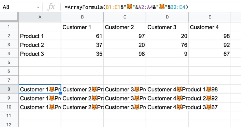
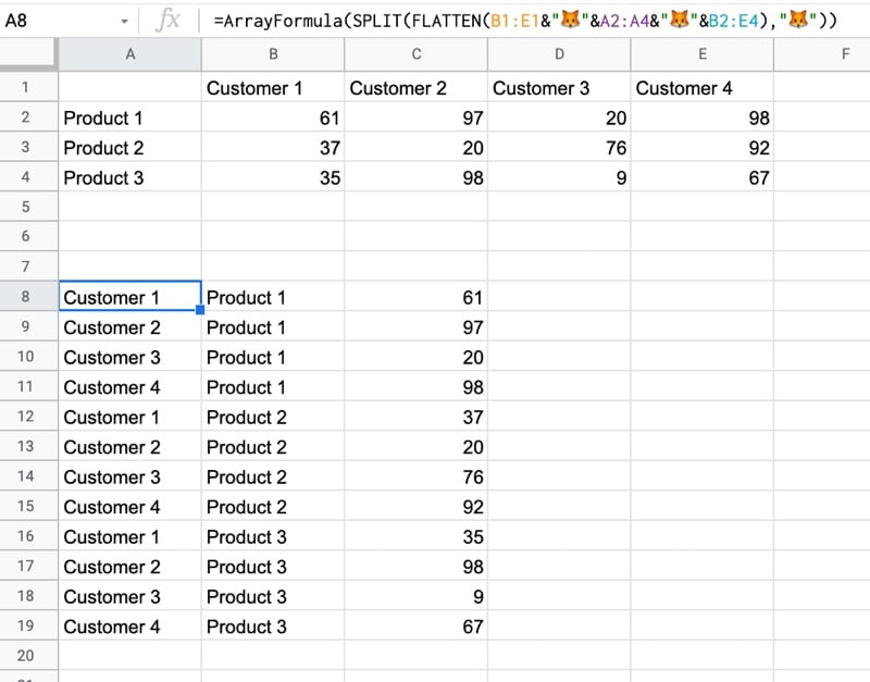
Use an array formula like this to combine the column headings (Customer 1, Customer 2, etc.) with the row headings (Product 1, Product 2, Product 3, etc.) and the data.
It’s crucial to add a special character between these sections of the dataset though, so we can split them up later on. I’ve used the fox emoji (because, why not?) but you can use whatever you like, provided it’s unique and doesn’t occur anywhere in the dataset.
=ArrayFormula(B1:E1&"🦊"&A2:A4&"🦊"&B2:E4)
The output of this formula is:
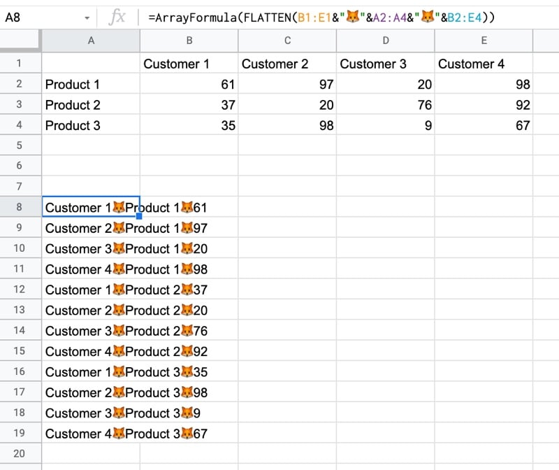
Step 2: Flatten The Data
Before the introduction of the FLATTEN function, this step was much, much harder, involving lots of weird formulas.
Thankfully the FLATTEN function does away with all of that and simply stacks all of the columns in the range on top of each other. So in this example, our combined data turns into a single column.
=ArrayFormula(FLATTEN(B1:E1&"🦊"&A2:A4&"🦊"&B2:E4))
The result is:
Step 3: Split The Data Into Columns
The final step is to split this new tall column into separate columns for each data type. You can see now why we needed to include the fox emoji so that we have a unique character to split the data on.
Wrap the formula from step 2 with the SPLIT function and set the delimiter to “🦊”:
I recently finished teaching my first cohort-based course, the first edition of Pro Sheets Accelerator.
Pro Sheets Accelerator is a live cohort-based course, where students go through the experience together over the course of 5 weeks. We had 37 students in this first cohort.
Rather than watching pre-recorded course videos alone, students met multiple times a week to learn together in a live setting on Google Meet. In addition, we had office hours, guest sessions, a community platform for Q&A, weekly recaps, templates, and replays of the live sessions online.
If video courses are all about the content and information, then cohort-based courses are all about community, accountability, and transformation.
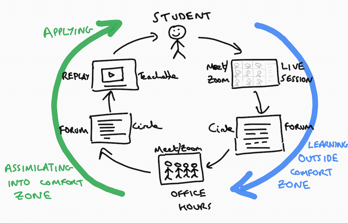
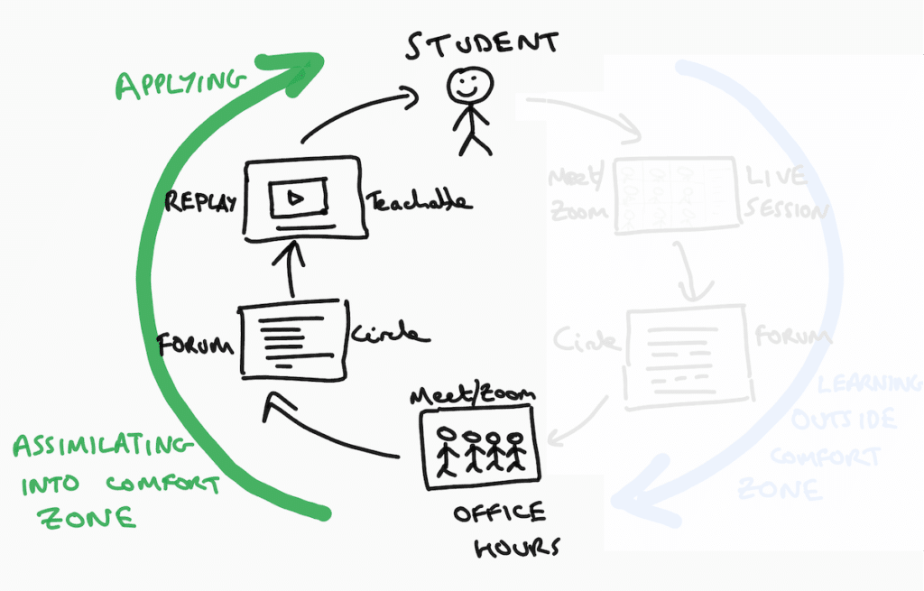
The Cohort-Based Course Student Learning Loop
Cohort-Based Course Student Learning Loop
The Student Learning Loop is a mechanism in your course to facilitate student transformations.
Cohort students pay a premium so they expect a premium outcome. They want to be transformed by the experience.
As the teacher/facilitator you have to create the mechanisms that enable students to have these transformative experiences.
There are countless videos on YouTube teaching your topic, so instead, you have to create an environment where students can undergo a transformation. Watching a YouTube video shows you a new technique. Attending a live session and participating gets you implementing a new technique. For many folks, this makes a big difference.
Let’s walk through the full cohort-based course Student Learning Loop, using specific examples from my Pro Sheets Accelerator course.
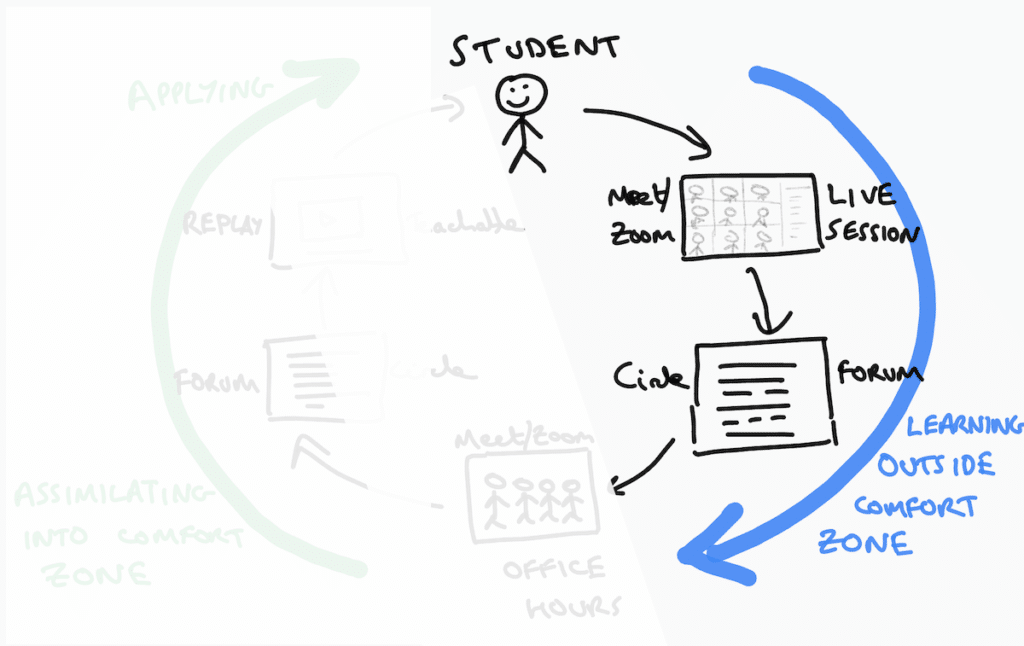
Student Learning Loop Phase 1: Learning
Learning happens in the first half of the Student Learning Loop, represented by the blue arc in this diagram:
Student Learning Loop Phase 1
The goal here is to get students into the zone of proximal development. To take them outside their comfort zones and stretch their abilities, but not so far that you lose them.
There’s a sweet spot where the majority of your students will be fully absorbed and learning.
There are two components in this phase:
live sessions
community forum for Q&A
Live Sessions
Pro Sheets Live Session 2
How do you conduct an engaging live session teaching technical topics via Google Meet or Zoom?
The key is to make it active with frequent state changes.
You can break up long slide monologues with demos, exercises, and breakout rooms.
Ben introduction to reinforce the journey and introduce the first new topic (10 minutes)
Ben live demo in a Google Sheet or Apps Script (10 minutes)
Student exercise (or breakout room) to practice themselves (20 minutes)
Topic consolidation and Q&A as a whole group (10 minutes)
Ben slides to introduce the second new topic (5 minutes)
Ben live demo of second new topic (10 minutes)
Second student exercise or breakout room (15 minutes)
Topic consolidation and Q&A as a whole group (5 minutes)
Closing discussion: recap what we learned today (5 minutes)
Frequent activities keep the students engaged, which makes for an effective learning environment.
Community Forum For Q&A
Hands up if you’ve thought of great questions after a live session?
Of course you have! We’ve all been there.
Not only that but some students aren’t comfortable asking questions in front of a group. And sometimes students miss a live session but still want to ask questions.
So it’s critical to have a place for students to ask questions about the materials asynchronously, outside the live sessions.
I use the community platform Circle to host the Pro Sheets Accelerator community. It’s an amazing tool that let me create a welcoming space for students to ask their questions.
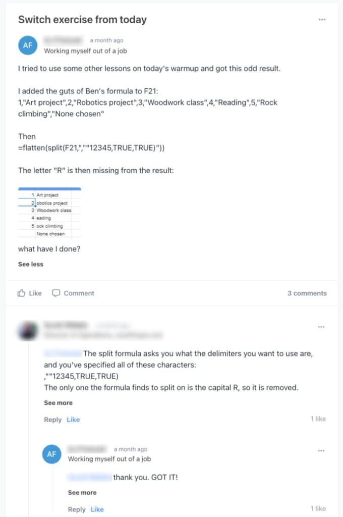
Here’s an example of the asynchronous learning process from Pro Sheets Accelerator:
IFS, SWITCH, and CHOOSE Functions Example
We covered the IFS function, SWITCH function, and CHOOSE function as part of session 4, in week 2. For many students, these were new functions so they were definitely outside their comfort zones during the live session demo and exercises.
After class, students practiced using these functions in their own work and could ask questions in our Circle forum:
Pro Sheets Circle Forum SWITCH function answer
In this particular example, a fellow student helped answer the question.
This peer coaching is another example of the value of cohort-based courses. Everyone is both a student and a teacher, bringing their own unique skills and experiences to the table.
Student Learning Loop Phase 2: Assimilation and Application
The second half of the Student Learning Loop happens when students incorporate information from the live sessions into their own workflows.
Both the office hours and the community forum help students do this effectively.
This is the second half of the Student Learning Loop, shown in green:
Student Learning Loop Phase 2
Student learning doesn’t stop once the lesson ends.
In fact, it’s really just the beginning.
True learning happens when students apply knowledge from the lessons to their own specific situations. Students benefit enormously from rapid feedback, so they don’t get stuck for long and learn quickly from their mistakes.
There are three components in this phase:
live office hours
more questions in the community forum
replays of live sessions
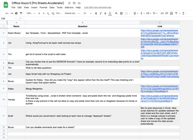
Live Office Hours
In Pro Sheets, we had live weekly office hours. These were 90-minute, drop-in, unstructured sessions where students could ask whatever questions they wanted.
They were a place for students to ask specific questions from their own domains.
We used a Google Sheet to collect questions, which then served as a repository of that knowledge for future reference.
Pro Sheets Office Hours Question Sheet
More Questions in the Community Forum
Throughout phase 2, students have lots of questions so the community plays an integral part in the assimilation and application of knowledge.
Students deepen their knowledge by asking and answering each other’s questions in the community forum.
Students also share their work wins with the community to get the validation they’re on track, which builds their confidence and reinforces the learning experience.
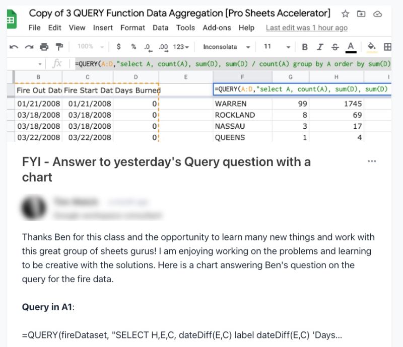
QUERY Function Example
For example, in week 2, I covered how to use the QUERY function to solve a challenging data analysis problem. The students were given a dataset of fires in New York State and asked to answer the question:
What is the average fire length in days, by county?
It was a challenging question because it required a query on top of another query (akin to a sub-query in SQL).
And here’s one student sharing their answer with the community:
Pro Sheets Circle Forum QUERY function answer
Replays and Templates
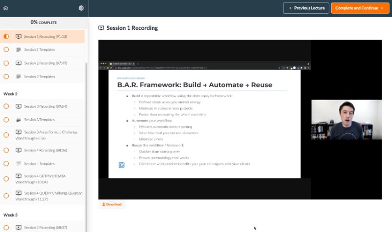
I use Teachable to host my on-demand video courses so it was a natural place to also host the video replays of the live session recordings for the Pro Sheets Accelerator course.
Teachable allows me to present the video recordings in a syllabus, with links to all of the template files.
Students have lifetime access to these video recordings and templates, so they can watch the live session replays and review topics as many times as they want.
This repetition helps cement the understanding.
Pro Sheets Session 1 replay on Teachable
Completing the Loop
Some students will progress through the loop multiple times a week, on the back of every live session. Others might progress at a slower pace and go through the loop once a week, whilst for others, it might happen a couple of times throughout the whole course.
Students undergo a transformation when they go through the learning loop. They return to work with new abilities and newfound confidence.
And that is the north star outcome we’re aiming for as course creators.
Evidence of A Transformation
“If you can’t measure it, you can’t improve it.” – Peter Drucker
Virtual high-fives during the final live session
I used Google Forms to conduct pre-course and post-course surveys, so I could measure and understand the transformation occurring at different stages of the Student Learning Loop framework.
In the post-course feedback form, I asked lots of questions, including what was the most valuable thing about the course, what they liked about the Circle community, the project, and the office hours. Here are some of the answers for Pro Sheets:
“It was great to work on a project during the week knowing that if I got stuck I could ask for help on Friday [office hours].”
“I’m really enjoying the course. I find myself thinking about the subject matter at odd hours, so it’s really taking root in my head.”
“Everyone in Circle was SO HELPFUL! And I loved seeing other peoples’ projects and questions. I got so many new ideas and perspectives. I also loved that in Circle we could build off of each others’ ideas. Like, the “Adding Notes” topic – you started with the basic idea but then so many people chimed in to make improvements. I have that script in at least 3 of my sheets now!”
“The workflow and BAR models are very useful concepts that I knew in a practical sense but needed to see more concretely. I feel like I moved forward on Array formulas, queries, custom functions, and Index-Match-Match.”
2024 Update: Table’s features and capabilities are now integrated into AppSheet. Read more here.
In this post, I’ll show you how to use the new Google Tables Apps Script Bot.
When something happens in your Google Table – a new row, or a value changes – a bot can be set to trigger an Apps Script function.
It opens up a world of new possibilities.
In this post, I’ll show you how to automatically enrich leads in Google Tables by retrieving data via the Mattermark API.
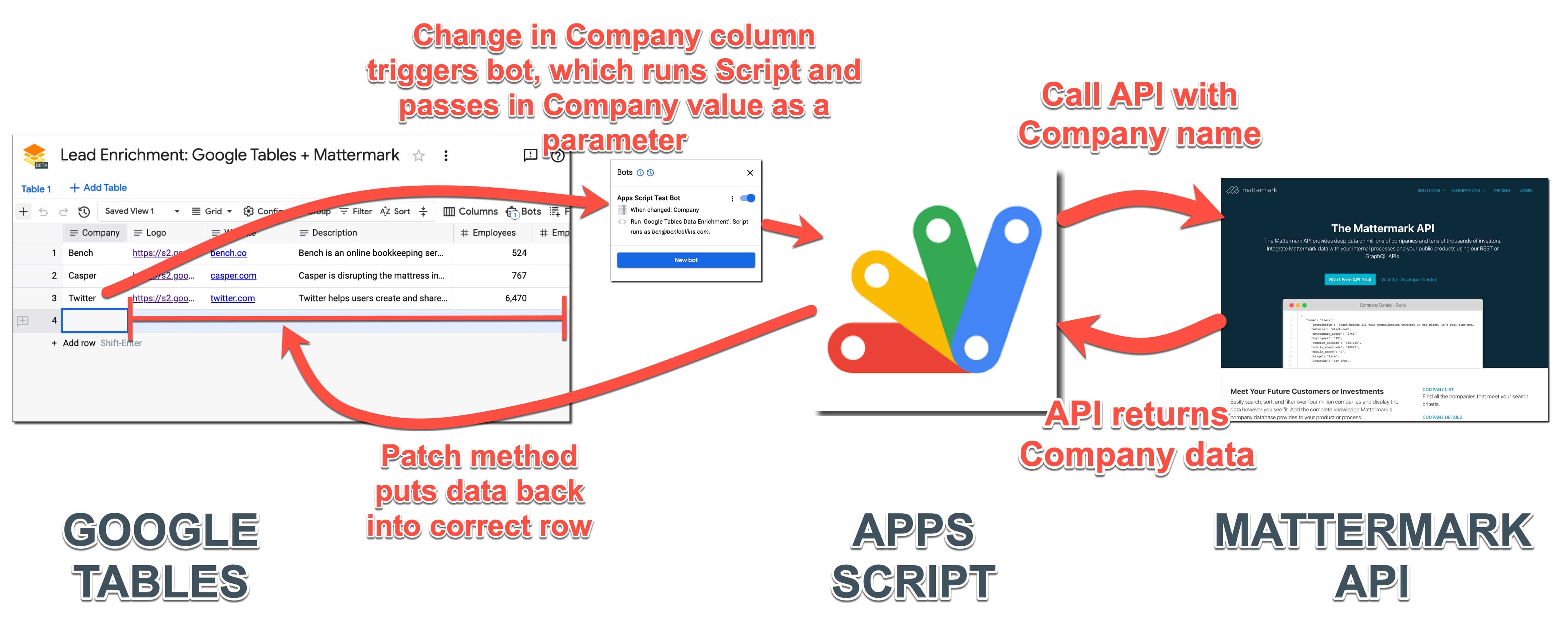
When I add a new company name into the first column, the new Google Tables Apps Script bot is triggered. The company name is passed to the Mattermark API and the relevant data is returned and finally added to that row in Google Tables.
Google Tables Apps Script Bot
Bots in Google Tables are automated actions that you do tasks for you, without needing to write any code.
Bots have three components:
Firstly, a trigger, which is a change in your Google Table that fires the bot
Secondly, any specific conditions that control the behavior of the bot, for example which rows it operates on
And thirdly, the action, i.e. what the bot does
It’s this third option where we can choose to run an Apps Script file as the bot action.
Google Tables Apps Script Bot Example: Data Enrichment
In this example, we’ll use data from the Mattermark API to enrich company data in our Google Table.
This is what the tool looks like in Google Tables:
When you type the company name, e.g. “Casper”, into the first column, the Google Tables Apps Script bot is triggered. This runs the Apps Script file and passes in the Company name as a parameter.
After that, the script file calls the Mattermark API with this company name and retrieves additional data for this company.
Finally, the script file adds this data back into the correct row of Google Tables using the PATCH method.
And here’s a flow chart of the overall workflow (click to enlarge):
Google Tables Set Up
The first step is to create a new Google Table with the following columns:
Column Heading
Data Type
Company
Text
Logo
Text
Website
Text
Description
Text
Employees
Number (integer)
Employees 6-Months Ago
Number (integer)
Revenue Range
Text
Website Uniques
Number (integer)
Mobile Downloads
Number (integer)
Funding Stage
Text
Total Funding
Number (integer)
City
Text
State
Text
Country
Text
Last updated
Update time
The only column that you’ll manually enter data into is the first column, Company, which holds the name of the company. The rest will all be populated by the script automatically (except the “Last updated” column which Tables takes care of).
Google Tables Bot
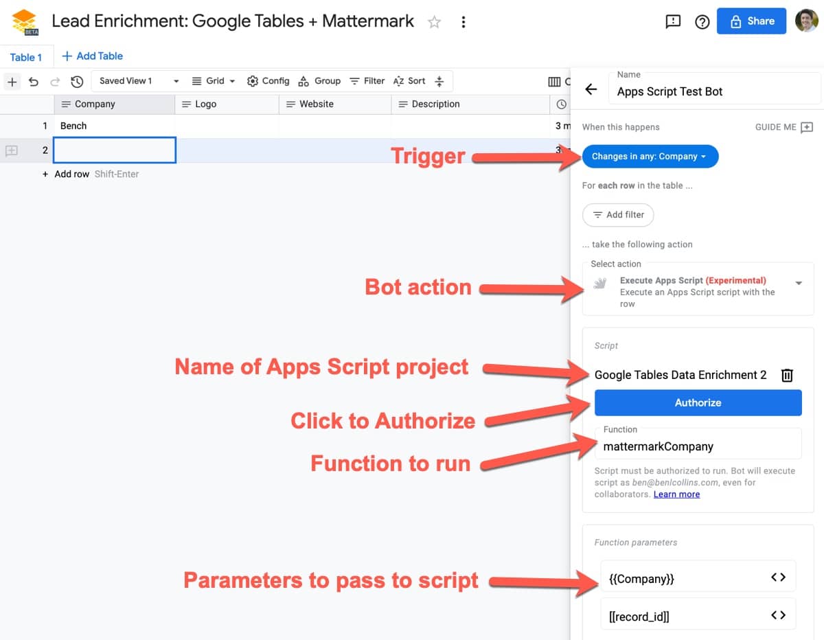
Next, create a bot with the following properties:
Trigger: Changes in any: Company
Action: Execute Apps Script
Then select the script file and function and authorize it (see below).
Function parameters: {{Company}} – so we can search for it on the Mattermark API [[record_id]] – the row ID for Google Tables so we can put the data back in the correct row
Here’s the bot setup in Google Tables (click to enlarge):
Find it in under Services on the left sidebar, then search for Area120Tables. Add it to your project.
Once you’ve added this Service, you’ll notice your appsscript.json manifest file has been updated to include it as an enabled advanced service.
Next, add this script to the editor:
/**
 * Global Variables
 */
const API_KEY = ''; // <-- enter your Mattermark API key here
const TABLE_NAME = ''; // <-- enter your Google Tables table ID here

/**
 * function to retrive logo url
 */
function retrieveCompanyLogoURL(companyWebsite) {

	// example
	// companyWebsite = 'bench.co'

	// setup the api
	const base = 'https://s2.googleusercontent.com/s2/favicons?domain=';
	const url = base + companyWebsite + '&sz=32';

	return url;

}

/**
 * function to retrieve company data from Mattermark
 */
function mattermarkCompany(companyName,recordID) {

	// example
	// companyName = 'facebook';

	// set up the api
	const base = 'https://api.mattermark.com/';
	const endpoint = 'companies/'
	const query = '?key=' + API_KEY + '&company_name=' + companyName;
	const url = base + endpoint + query;

	// call the api
	const response = UrlFetchApp.fetch(url);
	const data = JSON.parse(response.getContentText());

	// parse the data
	const companies = data.companies;
	const firstCompany = companies[0];
	const companyID = firstCompany.id;

	console.log(companies);
	console.log(firstCompany);
	console.log(companyID);

	// call the api to get specific company details
	mattermarkCompanyDetails(companyID,recordID);

}

/**
 * function to retrive company details
 */
function mattermarkCompanyDetails(companyID,recordID) {

	// example
	// companyID = '159108';

	// set up the api
	const base = 'https://api.mattermark.com/';
	const endpoint = 'companies/' + companyID;
	const query = '?key=' + API_KEY;
	const url = base + endpoint + query;

	// call the api
	const response = UrlFetchApp.fetch(url);
	const data = JSON.parse(response.getContentText());
	console.log(response.getResponseCode());
	//console.log(response.getContentText());

	// parse data
	const companyWebsite = data.website;
	const companyDescription = data.description;
	const companyEmployees = data.employees;
	const companyEmployeesSixMonthsAgo = data.employees_6_months_ago;
	const websiteUniques = data.website_uniques;
	const mobileDownloads = data.mobile_downloads;
	const fundingStage = data.stage;
	const totalFunding = data.total_funding;
	const city = data.city;
	const state = data.state;
	const country = data.country;
	const revenueRange = data.revenue_range;

	// add company logo data
	const companyLogo = retrieveCompanyLogoURL(companyWebsite);

	const enrichmentData = {
		'Logo': companyLogo,
		'Website': companyWebsite,
		'Description': companyDescription,
		'Employees': parseInt(companyEmployees),
		'Employees 6-Months Ago': parseInt(companyEmployeesSixMonthsAgo),
		'Revenue Range': revenueRange,
		'Website Uniques': parseInt(websiteUniques) || 0,
		'Mobile Downloads': parseInt(mobileDownloads) || 0,
		'Funding Stage': fundingStage,
		'Total Funding': parseInt(totalFunding),
		'City': city,
		'State': state,
		'Country': country
    };
    console.log(enrichmentData);

	// send data back to Google Tables
    const rowName = 'tables/' + TABLE_NAME + '/rows/' + recordID;
    Area120Tables.Tables.Rows.patch({values: enrichmentData}, rowName);

}
It’s a rough first draft! I’ve noted some improvements below.
Line 26: The mattermarkCompany function calls the API with the Company name to retrieve the Company ID.
It then calls mattermarkCompanyDetails function and passes in the Company ID.
Line 42: You’ll notice that I chose the first item of the company data array, regardless of whether this is the correct company. This was a shortcut to test out this idea.
Although this will often work, it won’t always grab the correct data because there could be multiple companies with the same name and you actually want the second one in the list. For a more robust tool, this would need to be developed further (noted in the improvements section below).
Line 57: The script calls the API again (a different endpoint) with this ID to get the additional data.
Subsequently, the script parses the returned data and puts it into an object (line 91).
Line 110: This line is the PATCH method to add the new data back into the correct row of my Google Table.
Script Improvements
There are a number of improvements that could be made:
Include error handling when no company data is found.
Deal with the multiple company scenario discussed above.
The Google Tables PATCH method could be moved into its own function, to further improve the code organization.
Include more data specific to the scenario (Mattermark has way more than I used in this example).
Sadly, I’ve used up my trial quota on the Mattermark API. Unfortunately, they only have annual plans available at over $1k, so for now, I’m not going to develop this any further.
In Summary
To sum up, the new Google Tables Apps Script bot is a great addition to Google Tables.
It opens up the door to all sorts of interesting automations with other Google Workspace tools or third-party services.
For example, suppose you have a Google Table of your employees and you add a new hire. This could trigger a bot that runs an Apps Script file to generate all the onboarding docs for that new employee, pre-filled with their data.
I’m excited to keep using it and see how else I can integrate Google Table automation into my workflows.
💡 Learn moreLearn how to write Apps Script and turbocharge your Google Workspace experience with the new Beginner Apps Script course
What is Google Apps Script?
Google Apps Script is a cloud-based scripting language for extending the functionality of Google Apps and building lightweight cloud-based applications.
It means you write small programs with Apps Script to extend the standard features of Google Workspace Apps. It’s great for filling in the gaps in your workflows.
With Apps Script, you can do cool stuff like automating repeatable tasks, creating documents, emailing people automatically and connecting your Google Sheets to other services you use.
Writing your first Google Script
In this Google Sheets script tutorial, we’re going to write a script that is bound to our Google Sheet. This is called a container-bound script.
(If you’re looking for more advanced examples and tutorials, check out the full list of Apps Script articles on my homepage.)
Hello World in Google Apps Script
Let’s write our first, extremely basic program, the classic “Hello world” program beloved of computer teaching departments the world over.
Begin by creating a new Google Sheet.
Then click the menu: Extensions > Apps Script
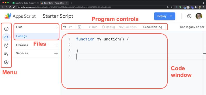
This will open a new tab in your browser, which is the Google Apps Script editor window:
By default, it’ll open with a single Google Script file (code.gs) and a default code block, myFunction():
function myFunction() {

}
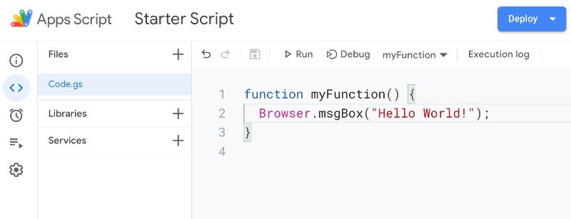
In the code window, between the curly braces after the function myFunction() syntax, write the following line of code so you have this in your code window:
function myFunction() {
  Browser.msgBox("Hello World!");
}
Your code window should now look like this:
Google Apps Script Authorization
Google Scripts have robust security protections to reduce risk from unverified apps, so we go through the authorization workflow when we first authorize our own apps.
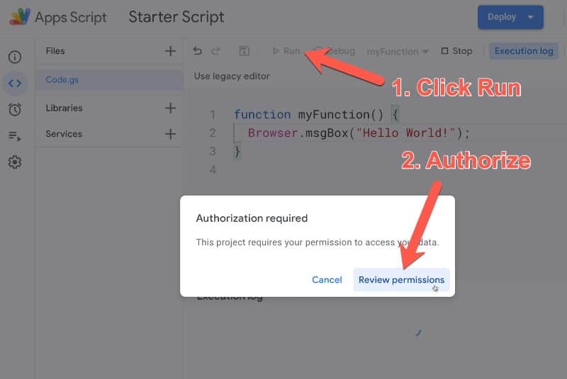
When you hit the run button for the first time, you will be prompted to authorize the app to run:
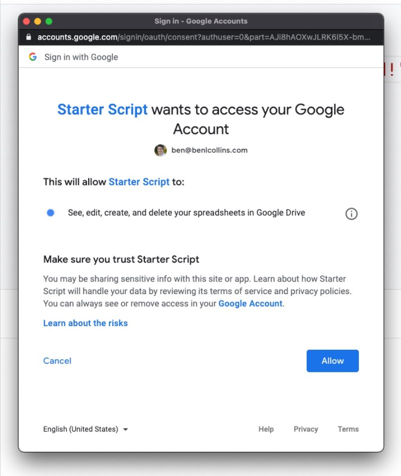
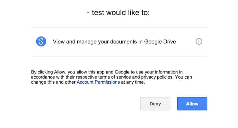
Clicking Review Permissions pops up another window in turn, showing what permissions your app needs to run. In this instance the app wants to view and manage your spreadsheets in Google Drive, so click Allow (otherwise your script won’t be able to interact with your spreadsheet or do anything):
❗️When your first run your apps script, you may see the “app isn’t verified” screen and warnings about whether you want to continue.
In our case, since we are the creator of the app, we know it’s safe so we do want to continue. Furthermore, the apps script projects in this post are not intended to be published publicly for other users, so we don’t need to submit it to Google for review (although if you want to do that, here’s more information).
Click the “Advanced” button in the bottom left of the review permissions pop-up, and then click the “Go to Starter Script Code (unsafe)” at the bottom of the next screen to continue. Then type in the words “Continue” on the next screen, click Next, and finally review the permissions and click “ALLOW”, as shown in this image (showing a different script in the old editor):
Once you’ve authorized the Google App script, the function will run (or execute).
If anything goes wrong with your code, this is the stage when you’d see a warning message (instead of the yellow message, you’ll get a red box with an error message in it).
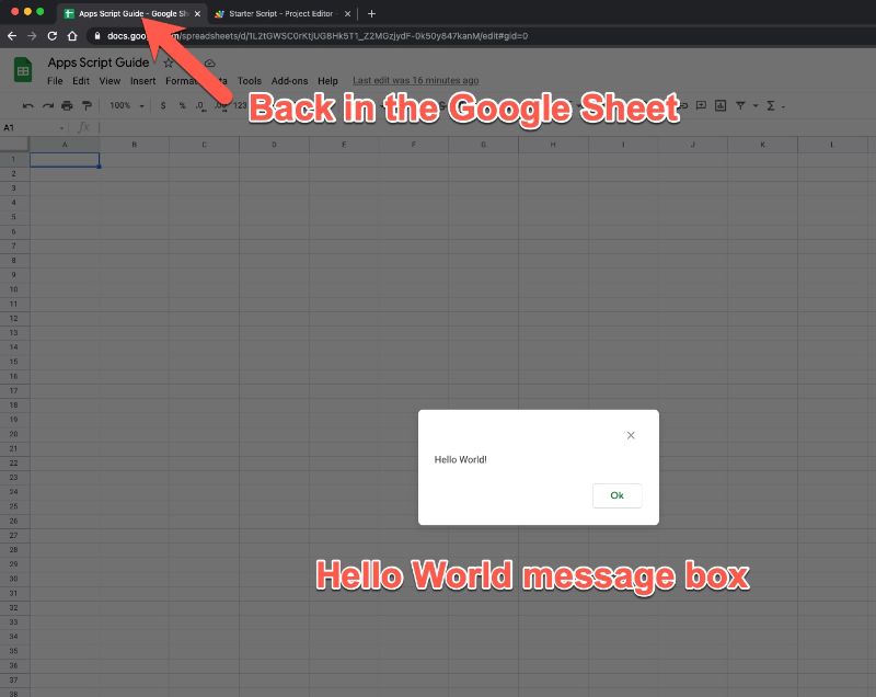
Return to your Google Sheet and you should see the output of your program, a message box popup with the classic “Hello world!” message:
Click on Ok to dismiss.
Great job! You’ve now written your first apps script program.
Rename functions in Google Apps Script
We should rename our function to something more meaningful.
At present, it’s called myFunction which is the default, generic name generated by Google. Every time I want to call this function (i.e. run it to do something) I would write myFunction(). This isn’t very descriptive, so let’s rename it to helloWorld(), which gives us some context.
So change your code in line 1 from this:
function myFunction() {
  Browser.msgBox("Hello World!");
}
to this:
function helloWorld() {
  Browser.msgBox("Hello World!");
}
Note, it’s convention in Apps Script to use the CamelCase naming convention, starting with a lowercase letter. Hence, we name our function helloWorld, with a lowercase h at the start of hello and an uppercase W at the start of World.
Adding a custom menu in Google Apps Script
In its current form, our program is pretty useless for many reasons, not least because we can only run it from the script editor window and not from our spreadsheet.
Let’s fix that by adding a custom menu to the menu bar of our spreadsheet so a user can run the script within the spreadsheet without needing to open up the editor window.
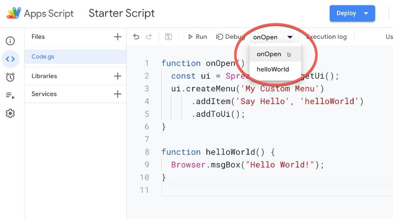
This is actually surprisingly easy to do, requiring only a few lines of code. Add the following 6 lines of code into the editor window, above the helloWorld() function we created above, as shown here:
If you look back at your spreadsheet tab in the browser now, nothing will have changed. You won’t have the custom menu there yet. We need to re-open our spreadsheet (refresh it) or run our onOpen() script first, for the menu to show up.
To run onOpen() from the editor window, first select then run the onOpen function as shown in this image:
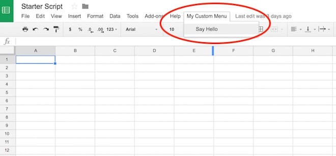
Now, when you return to your spreadsheet you’ll see a new menu on the right side of the Help option, called My Custom Menu. Click on it and it’ll open up to show a choice to run your Hello World program:
Run functions from buttons in Google Sheets
An alternative way to run Google Scripts from your Sheets is to bind the function to a button in your Sheet.
For example, here’s an invoice template Sheet with a RESET button to clear out the contents:
Another great way to get started with Google Scripts is by using Macros. Macros are small programs in your Google Sheets that you record so that you can re-use them (for example applying standard formatting to a table). They use Apps Script under the hood so it’s a great way to get started.
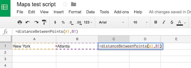
Let’s create a custom function with Apps Script, and also demonstrate the use of the Maps Service. We’ll be creating a small custom function that calculates the driving distance between two points, based on Google Maps Service driving estimates.
The goal is to be able to have two place-names in our spreadsheet, and type the new function in a new cell to get the distance, as follows:
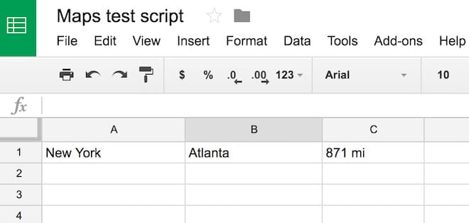
The solution should be:
Copy the following code into the Apps Script editor window and save. First time, you’ll need to run the script once from the editor window and click “Allow” to ensure the script can interact with your spreadsheet.
function distanceBetweenPoints(start_point, end_point) {
  // get the directions
  const directions = Maps.newDirectionFinder()
     .setOrigin(start_point)
     .setDestination(end_point)
     .setMode(Maps.DirectionFinder.Mode.DRIVING)
     .getDirections();

  // get the first route and return the distance
  const route = directions.routes[0];
  const distance = route.legs[0].distance.text;
  return distance;
}
Saving data with Google Apps Script
Let’s take a look at another simple use case for this Google Sheets Apps Script tutorial.
Suppose I want to save copy of some data at periodic intervals, like so:
In this script, I’ve created a custom menu to run my main function. The main function, saveData(), copies the top row of my spreadsheet (the live data) and pastes it to the next blank line below my current data range with the new timestamp, thereby “saving” a snapshot in time.
The code for this example is:
// custom menu function
function onOpen() {
  const ui = SpreadsheetApp.getUi();
  ui.createMenu('Custom Menu')
      .addItem('Save Data','saveData')
      .addToUi();
}

// function to save data
function saveData() {
  const ss = SpreadsheetApp.getActiveSpreadsheet();
  const sheet = ss.getSheets()[0];
  const url = sheet.getRange('Sheet1!A1').getValue();
  const follower_count = sheet.getRange('Sheet1!B1').getValue();
  const date = sheet.getRange('Sheet1!C1').getValue();
  sheet.appendRow([url,follower_count,date]);
}
2. Open script editor from the menu: Extensions > Apps Script
3. In the newly opened Script tab, remove all of the boilerplate code (the “myFunction” code block)
4. Copy in the following code:
// code to add the custom menu
function onOpen() {
  const ui = DocumentApp.getUi();
  ui.createMenu('My Custom Menu')
      .addItem('Insert Symbol', 'insertSymbol')
      .addToUi();
}

// code to insert the symbol
function insertSymbol() {
  // add symbol at the cursor position
  const cursor = DocumentApp.getActiveDocument().getCursor();
  cursor.insertText('§§');

}
5. You can change the special character in this line
cursor.insertText('§§');
to whatever you want it to be, e.g.
cursor.insertText('( ͡° ͜ʖ ͡°)');
6. Click Save and give your script project a name (doesn’t affect the running so call it what you want e.g. Insert Symbol)
7. Run the script for the first time by clicking on the menu: Run > onOpen
8. Google will recognize the script is not yet authorized and ask you if you want to continue. Click Continue
9. Since this the first run of the script, Google Docs asks you to authorize the script (I called my script “test” which you can see below):
10. Click Allow
11. Return to your Google Doc now.
12. You’ll have a new menu option, so click on it:
My Custom Menu > Insert Symbol
13. Click on Insert Symbol and you should see the symbol inserted wherever your cursor is.
Google Apps Script Tip: Use the Logger class
Use the Logger class to output text messages to the log files, to help debug code.
The log files are shown automatically after the program has finished running, or by going to the Executions menu in the left sidebar menu options (the fourth symbol, under the clock symbol).
The syntax in its most basic form is Logger.log(something in here). This records the value(s) of variable(s) at different steps of your program.
For example, add this script to a code file your editor window:
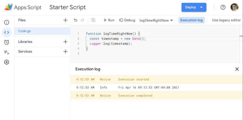
function logTimeRightNow() {
  const timestamp = new Date();
  Logger.log(timestamp);
}
Run the script in the editor window and you should see:
Real world examples from my own work
I’ve only scratched the surface of what’s possible using G.A.S. to extend the Google Apps experience.
Here are a couple of interesting projects I’ve worked on:
1) A Sheets/web-app consisting of a custom web form that feeds data into a Google Sheet (including uploading images to Drive and showing thumbnails in the spreadsheet), then creates a PDF copy of the data in the spreadsheet and automatically emails it to the users. And with all the data in a master Google Sheet, it’s possible to perform data analysis, build dashboards showing data in real-time and share/collaborate with other users.
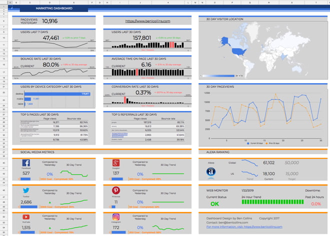
2) A dashboard that connects to a Google Analytics account, pulls in social media data, checks the website status and emails a summary screenshot as a PDF at the end of each day.
Imagination and patience to learn are the only limits to what you can do and where you can go with GAS. I hope you feel inspired to try extending your Sheets and Docs and automate those boring, repetitive tasks!
The IFS function in Google Sheets is used to test multiple conditions and outputs a value specified by the first test that evaluates to true.
It’s akin to a nested IF formula, although it’s not exactly the same. However, if you find yourself creating a nested IF formula then it’s probably easier to use this IFS function.