Let’s hope for a brighter, happier, safer lap around the sun this time.
We had a December snowstorm! Lots of fun with the young ‘uns 🙂
This is annual review number 6!
As always, I’m super grateful when I sit down to write this because it means I’m still working for myself and building this business.
2020 was a difficult year for the world.
I’m fortunate to have my health and so do those close to me. I can’t imagine how difficult 2020 has been for those who have lost someone. My heart goes out to you.
My wife and I have taken the virus seriously. Given my history of pneumonia in the last two years (see challenges of 2018 and 2019) I can’t afford to take this virus lightly.
We’re extremely fortunate that we already work from home, so that didn’t present a significant challenge when the whole world went remote. However, going from full time childcare to no childcare was certainly a challenge.
I’m looking forward to 2021 and the promise of a vaccine. I haven’t seen my UK family since January 2020 and I miss them (and the UK) terribly.
I’m cautiously optimistic that 2021 will be better, and make up for the annus horribilis that was 2020.
With that, let me present my review of the year:
Did I Meet My 2020 Goals?
Overall, given the circumstances – I probably had 50% fewer working hours this year because I spent that time with my kids – I’m really happy with what I achieved and feel positive about how the year went from a work perspective.
Publish more high-quality tutorials than in 2019 (target > 17) – Yes! I wrote 26 new tutorials this year.
Hit 50k newsletter subscribers and send out a tip every Monday – Yes and no. I sent a newsletter every Monday and hit 40k subs, which I’m super happy with. This is after removing 8k inactive subs, so I actually got pretty close to my original goal.
Update my existing Google Sheets courses – Yes! I re-recorded all of the Google Sheet course videos. I’m updating the Automation with Apps Script course at the moment, which will complete the update process.
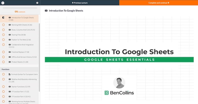
Create one new Google Sheets course – Yes! I launched the Google Sheets Essentials course this year.
Run 10 in-person workshops – No. Obviously not 😉
Re-brand my digital assets – Yes! I was thrilled with how it turned out. Details below.
Find a VA to help with the business – Yes! And she’s been an enormous help. Thanks, Jo!
Live-blog Google Next 2020 again – No 🙁 Obviously, this didn’t happen since the conference was cancelled.
Work through this book: Data Science on the Google Cloud Platform – Sort of. I started the book and worked through another BigQuery book, but it’s still early in that journey.
My overall number 1 goal for 2020 is to be healthy – Yes! Apart from my whole family having the flu in February and a grotty headcold in August, I’ve been healthy this year.
Fitness goals: be active 5 times/week (a mix of spin classes, runs and at least 1 run/hike up the mountain) – Sort of… my R knee is still not healed from the running injuries last year, so I’ve been confined to hiking and occasional yoga classes.
Keep up the weekly brainstorming hike with my wife – The pandemic put a dampener on this. We’ve managed a few hikes together but since childcare is limited in the current circumstances, we haven’t had the opportunity to do this weekly as we’d hoped.
Read 30 books – No. I read ~20 books, but the last one I read was 650 pages of small print, all about life in Stalin’s Russia of the 1930s, 40s and 50s. That counts for at least 3 or 4 normal books by my reckoning 😉
2020 Highlights
2020 felt like a long year. Events from the start of this year feel like they happened years ago. I feel like I aged 10 years!
But despite the terrible toll the pandemic exacted on us all, there were plenty of highlights throughout the year.
In no particular order:
1) New Brand
I hired the super talented team at Left Hand Design to do a rebrand for my business and courses.
I wanted something simple, bold and geometric, and I think Left Hand Design did an outstanding job.
Over the course of a couple of months, they created new family of logos, new color scheme, fonts and styles for my entire online presence. They created new images for my courses and a new slide deck template for the lessons.
I also need to credit my wife, Alexis Grant, for the green dot over the “i”, a wonderful addition!
This new brand represents a huge leap forward for my business.
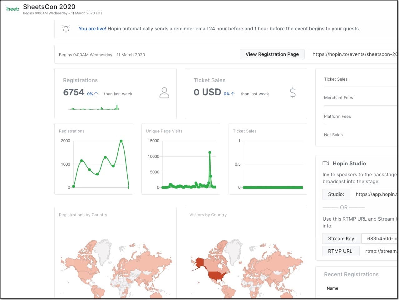
2) SheetsCon
In March this year I ran my most ambitious project to date: SheetsCon, a 2-day online conference for all things Google Sheets.
When I planned the conference in late 2019, way before any of us had heard of Coronavirus, I envisioned an online conference so that people from all over the world could participate, free of charge.
SheetsCon ran on Wednesday 11th and Thursday 12th March. My sons had their last day at preschool on the 13th March, because it shut down the following week. We all went into lockdown that weekend.
The timing of an online conference in March might have looked prescient from the outside, but I can promise you it wasn’t planned that way because of Covid.
The event was a massive success; we had almost 7,000 registered attendees, 3,800 of whom attended live, and 89.5% of whom said they’ll return in 2021.
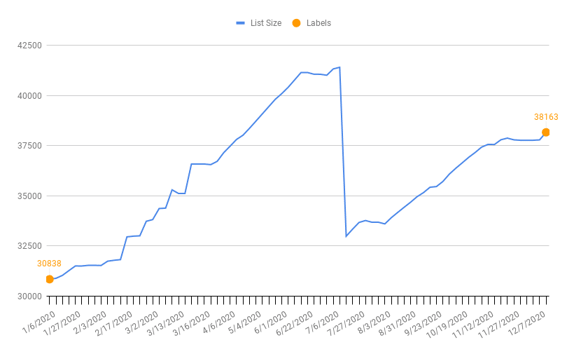
My email list has grown from around 30,000 at the beginning of the year to over 38,000 by year end, after removing over 8,000 inactive subscribers part way through the year (the steep drop).
Email continues to be my main marketing channel, and the list grew steadily throughout the year. I get about 40 – 50 daily signups for the Google Sheets Tips newsletter, which goes out at 11am every Monday.
I sent 51 Google Sheets Tips newsletters this year, only skipping the Christmas week.
I’m grateful to all of you who read this website, open my Google Sheets tips newsletters or learn from one of my online courses. It’s a great privilege to share my teachings with the world. I love my work and hope to serve you for years to come. Thank you! 🙏
I’m also extremely grateful to the Google Developer Expert Workspace group and the Googlers I’ve gotten to know over the past few years. It’s been a real pleasure to learn from you all and I’m humbled to be included in such a wonderful and knowledgeable group. Cheers to future collaborations!
Spending lots of time with my two young sons this year and watching them blossom, despite the difficult circumstances. Yes, it’s been frustrating and challenging at times, but it’s impossible to put into words how much I love these two little guys and want to do my best for them.
We had a wonderful week at Deep Creek Lake with my wife’s family in August. It was relaxing and we got to be mostly normal for a week, and socialize with more than just my immediate family four. We enjoyed time on the lake, some great hikes, fires and BBQs!
2020 was an incredibly challenging year for everyone. I’m grateful that I, and those close to me, have remained healthy this year.
Aside from staying healthy and isolating, the biggest challenge for my wife and me was the lack of childcare.
We had no childcare in April or May, some in June to August, and then about 28 hours/week since September-ish. Since we both have our own businesses and are ambitious, it’s been a tricky balancing act.
Looking Forward To 2021
I’m super focussed on doing just a few things as well as I can, so I condensed my entire 2021 plan onto a single whiteboard.
Obviously, this only covers the big ticket items, and not things like the blog posts. I find it incredibly helpful to have it written down though. I look at every day to keep me focussed.
New Initiatives
My big initiative for 2021 is to create a cohort-based course for Google Sheets and data analysis, tentatively called ProSheets.
It’ll consist of two live classes and office hours each week for 5 weeks, with a project to finish. You’ll be in a cohort with other students going through the same transformation, so you’ll have a peer group to be accountable with. You’ll leave the course as a pro with Google Sheets, how to solve business and data analysis problems from end-to-end, and have an amazing group of peers to continue learning with. More details to come in early 2021!
To make this new course as successful as possible for students, I’m joining two training programs myself in early 2021. They are: 1) the Keystone Accelerator course, a course/mastermind with other ambitious creators looking to start cohort courses, and 2) the Scaling Intimacy workshop, all about how to create memorable online experiences. I’m super excited about both and can’t wait to put these lessons into practice.
2021 Work Goals
Run 3 cohorts of this new live cohort based course
Publish a comprehensive guide to REGEX in Google Sheets
Hit 60k newsletter subscribers
Send a Google Sheets tip email every week for the next year
Create one new on-demand video course
One technical project, related to Sheets/Apps Script/Data in some way. This is partly for my own intellectual curiosity and learning but will also lay the foundations for future blog posts and courses.
Other 2021 Goals
See my UK family!
Have another healthy year
Exercise regularly: 4 hike or bikes each week, 2 yoga/strength
Go camping again! I used to do a lot of camping but it’s been a few years since I last went 🙁
Take my boys out on lots of adventures and camping trips.
Read 30 books (same target as 2020)
Thank You
Finally, my biggest thanks are reserved for you, dear reader.
It’s an extreme honor and privilege for me to help you through my writing and teaching.
My work to create the world’s best resources for learning Google Sheets and data analysis is just getting started.
Growing up, I vividly remember sitting in my dad’s home office after school, waiting for him to get home from work.
The office had a tall ceiling and a single window at the back that opened into a tiny access courtyard between our house and the neighbor’s house (it was a semi-detached Victorian).
My dad sat behind a heavy wooden desk, with a big, boxy desktop computer sitting atop. On one wall was a bookshelf, full of computer books and boxes of floppy disks for illustrious programs like Microsoft Windows, Lotus 1-2-3, Borland Quattro Pro, and many others I’ve forgotten.
I would pull the thickest manual off the shelf and ask dad to explain it to me the minute he got home from work. I’m sure it’s just what he wanted to do at the end of a long work day. Sorry (but not sorry) dad!
I’ve wanted my own work space, reflecting my personality and overflowing with books, ever since.
Working From Home
I’ve worked for myself for 5 years now, so I’m used to working from home.
For the first couple of years, I worked from a small desk in the living room and then the basement of where I lived at the time.
When my wife and I moved to Florida in 2017, I rented a 1-person office in downtown St. Petersburg. My youngest son was only a few months old so I needed a quiet space to record videos. (I launched my first online course in 2017.)
I customized that rental office to make it my own. The first investment was a Fully Jarvis standing desk, which I still use and love today.
Last year, we moved to Harpers Ferry, WV, and it was a chance to set up a new office. The only change was the better scenery out my window and a couple of pieces of artwork on the walls.
This year, 2020, we moved out of the rental house and into our own home, so it was finally time to build the dream office. This is iteration three of my home office.
An Investment In You And Your Business
I’ve come to realize that the environment in which you do your work is important.
To do my best work I need to clear my mind out first. If there’s clutter everywhere, which is most days since I have young kids, then my mind is using energy to think about it. In my head, I’m doing a virtual Maire Kondo where I sweep it all away and out of sight.
My office is one space I have control over though. I can set it up to be clean and minimal.
Today, I’m much more sure of who I am and what I do than at any previous stage in life. And that translates into being able to create a workspace that facilitates the work I do now.
Global HQ for Collins Analytics LLC
My 2014 MacBook Pro is 6 years old and showing its age.
I don’t do a lot of heavy-duty computing, but I do work with large video files. And of course, I have a lot of Chrome tabs open at any given time.
The time from deciding I needed a new computer to actually purchasing one was about 12 months!
I spent a LOT of time researching options and looking at other’s setups.
I’m using the new Apple Mac Mini with the M1 chip, powering 2 monitors: an ultrawide Dell U3419W (supported by a Fully Jarvis monitor arm) and an Acer R240HY.
The microphone is a Blue Yeti on a Blue Compass arm, and the light is an Elgato Key light.
Everything sits on Fully’s Jarvis standing desk, which I’ve had for years and love.
So far, it’s a fantastic combination! Super fast, quiet and tons of real estate.
That’s a Lego Saturn V rocket on the window ledge, one of the greatest Lego models of all time.
This tutorial is written for Google Sheets users who have datasets that are too big or too slow to use in Google Sheets. It’s written to help you get started with Google BigQuery.
If you’re experiencing slow Google Sheets that no amount of clever tricks will fix, or you work with datasets that are outgrowing the 10 million cell limit of Google Sheets, then you need to think about moving your data into a database.
As a Google user, probably the best and most logical next step is to get started with Google BigQuery and move your data out of Google Sheets and into BigQuery.
By the end of this tutorial, you will have created a BigQuery account, uploaded a dataset from Google Sheets, written some queries to analyze the data and exported the results back to Google Sheets to create a chart.
You’ll also do the same analysis side-by-side in a Google Sheet, so you can understand exactly what’s happening in BigQuery.
I’ve highlighted the action steps throughout the tutorial, to make it super easy for you to follow along:
Google BigQuery exercise steps are shown in blue.
Actions for you to do in Google BigQuery.
Google Sheet exercise steps are shown in green.
Actions for you to do in Google Sheets.
Section 1: What is BigQuery?
Google BigQuery is a data warehouse for storing and analyzing huge amounts of data.
Officially, BigQuery is a serverless, highly-scalable, and cost-effective cloud data warehouse with an in-memory BI Engine and machine learning built in.
This is a formal way of saying that it’s:
Works with any size data (thousands, millions, billions of rows…)
Easy to set up because Google handles the infrastructure
Grows as your data grows
Good value for money, with a generous free tier and pay-as-you-go beyond that
Lightning fast
Seamlessly integrated with other Google tools, like Sheets and Data Studio
Can import and export data from and to many sources
Has Built-in machine learning, so predictive modeling can be set up quickly
What’s the difference between BigQuery and a “regular” database?
BigQuery is a database optimized for storing and analyzing data, not for updating or deleting data.
It’s ideal for data that’s generated by e-commerce, operations, digital marketing, engineering sensors etc. Basically, transactional data that you want to analyze to gain insights.
A regular database is suitable for data that is stored, but also updated or deleted. Think of your social media profile or customer database. Names, emails, addresses, etc. are stored in a relational database. They frequently need to be updated as details change.
Section 2: Google BigQuery Setup
It’s super easy to get started wit Google BigQuery!
There are two ways to get started: 1) use the free sandbox account (no billing details required), or 2) use the free tier (requires you to enter billing details, but you’ll also get $300 free Cloud credits).
In either case, this tutorial won’t cost you anything in BigQuery, since the volume of data is so tiny.
We’ll proceed using the sandbox account, so that you don’t have to enter any billing details.
A new project called “My First Project” is automatically created
In the left side pane, scroll down until you see BigQuery and click it
Here’s that process shown as a GIF:
You’re ready for Step 2 below.
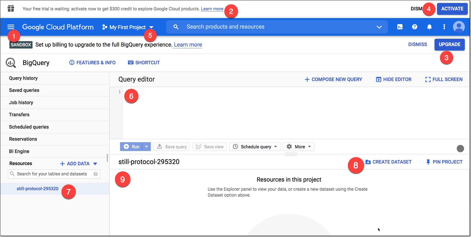
BigQuery Console
(click to enlarge)
Here’s what you can see in the console:
The SANDBOX tag to tell you you’re in the sandbox environment
Message to upgrade to the free trial and $300 credit (may or may not show)
UPGRADE button to upgrade out of the Sandbox account
ACTIVATE button to claim the free $300 credit
The current project and where to create new projects
The Query editor window where you type your SQL code
Current project resource
Button to create a new dataset for this project (see below)
Query outputs and table information window
What is the free Sandbox Account?
The sandbox account is an option that lets you use BigQuery without having to enter any credit card information. There are limits to what you can do, but it gives you peace of mind that you won’t run up any charges whilst you’re learning.
In the sandbox account:
Tables or views last 60 days
You get 10 Gb of storage per month for free
And 1 Tb data processing each month
It’s more than enough to do everything in this tutorial today.
Unlike Google Sheets, you have to pay to use BigQuery based on your storage and processing needs.
However, there is a sandbox account for free experimentation (see below) and then a generous free tier to continue using BigQuery.
In fact, if you’re working with datasets that are only just too big for Sheets, it’ll probably be free to use BigQuery or very cheap.
BigQuery charges for data storage, streaming inserts, and for querying data, but loading and exporting data are free of charge.
Your first 1 TB (1,000 GB) per month is free.
Full BigQuery pricing information can be found here.
Clicking on the blue “Try BigQuery free” button on the BigQuery homepage will let you register your account with billing details and claim the free $300 cloud credits.
Section 3: How to get your data into BigQuery
Extracting, loading and transforming (ELT) is sometimes the most challenging and time consuming part of a data analysis project. It’s the most engineering-heavy stage, where the heavy lifting happens.
You can load data into BigQuery in a number of ways:
From a readable data source (such as your local machine)
From Google Sheets
From other Google services, such as Google Ad Manager and Google Ads
Use a third-party data integration tool, e.g. Supermetrics, Stitch
You might want to make a SECOND copy in your Drive folder too, so you can keep one copy untouched for the upload to BigQuery and use the second copy for doing the follow-along analysis in Google Sheets.
The first dataset is a record of pedestrian traffic crossing Brooklyn Bridge in New York city (source).
It’s only 7,000 rows, so it could be easily analyzed in Sheets of course, but we’ll use it here so that you can do the same steps in BigQuery and in Sheets.
The second dataset is a daily total of bike counts for New York’s East River bridges (source).
There’s nothing inherently wrong with putting “small” data into BigQuery. Yes, it’s designed for truly gigantic datasets (billions of rows+) but it works equally well on data of any size.
Back in the BigQuery Console, you need to set up a project before you can add data to it.
Get started with Google BigQuery: Loading data From A Google Sheet
Think of the Project as a folder in Google Drive, the Dataset as a Google Sheet and the Table as individual Sheet within that Google Sheet.
The first step to get started with Google BigQuery is to create a project.
In step 1, BigQuery will have automatically generated a new project for you, called “My First Project”.
If it didn’t, or you want to create another new project, here’s how.
Step 3: Create a new Project
In the top bar, to the right of where it says “Google Cloud Platform”, click on Project drop-down menu.
In the popup window, click NEW PROJECT.
Give it a name, organization (your domain) and location (parent organization or folder).
Optionally, you can choose to bookmark this project in the Resources section of the sidebar. Click “PIN PROJECT” to do this.
Step 4: Create a new Dataset
Next you need to create a dataset by clicking “CREATE DATASET“.
Name it “start_bigquery”. You’re not allowed to have any spaces or special characters apart from the underscore.
Set the data location to your locale, leave the other settings alone and then click “Create dataset”
This new dataset will show up underneath your project name in the sidebar.
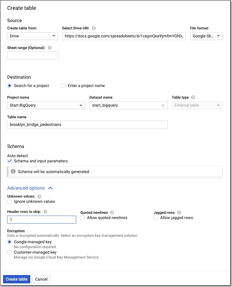
Step 5: Create a new Table
With the dataset selected, click on the “+ CREATE TABLE” or big blue plus button.
You want to select “Drive”, add the URL and set the file format to Google Sheets.
Name your table “brooklyn_bridge_pedestrians”.
Choose Auto detect schema.
Under Advanced settings, tell BigQuery you have a single header row to skip by entering the value 1.
Your settings should look like this:
If you make a mistake, you can simply delete the table and start again.
Section 4: Analyzing Data in BigQuery
Google BigQuery uses Structure Query Language (SQL) to analyze data.
The Google Sheets Query function uses a similar SQL style syntax to parse data. So if you know how to use the Query function then you basically know enough SQL to get started with Google BigQuery!
Basic SQL Syntax for BigQuery
The basic SQL syntax to write queries looks like this:
SELECT these columns
FROM this table
WHERE these filter conditions are true
GROUP BY these aggregate conditions
HAVING these filters on aggregates
ORDER BY i.e. sort by these columns
LIMIT restrict answer to X number of rows
You’ll see all of these keywords and more in the exercises below.
Get started with Google BigQuery: First Query
The BigQuery console provides a button that gives you a starter query.
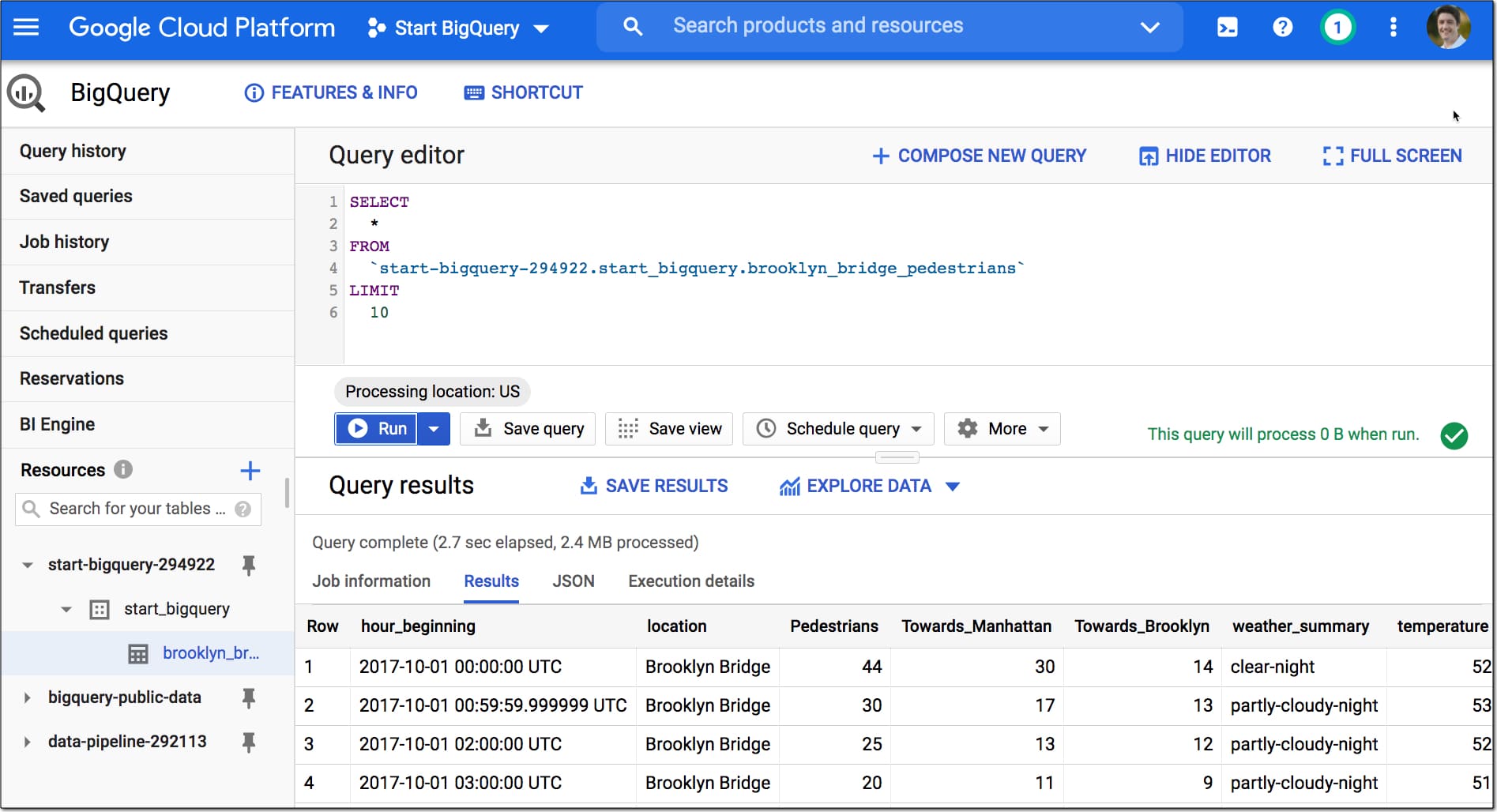
Step 6: Write your first query
Click on “QUERY TABLE” and this query shows up in your editor window:
SELECT FROM `start-bigquery-294922.start_bigquery.brooklyn_bridge_pedestrians` LIMIT 1000
Modify it by adding a * between the SELECT and FROM, and reducing the number after LIMIT to 10:
SELECT
  *
FROM
  `start-bigquery-294922.start_bigquery.brooklyn_bridge_pedestrians`
LIMIT
  10
Then format your query across multiple lines with through the menu: More > Format
SELECT
*
FROM
`start-bigquery-294922.start_bigquery.brooklyn_bridge_pedestrians`
LIMIT
10
Click “▶️ Run” to execute the query.
The output of this query will be 10 rows of data showing under the query editor:
(click to enlarge)
Woohoo!
You just wrote your first query in Google BigQuery.
Let’s continue and analyze the dataset:
Exercise 2: Analyzing Data In BigQuery
Run through the following steps:
Step 7: tell the story of one row
I always advocate doing this with any new dataset.
Write a query that selects all the columns (SELECT *) and a limited number of rows (e.g. LIMIT 10), as you did in step 6 above.
Run that query and look at the output. Scan across one whole row. Look at every column and think about what data is stored there.
Think about doing the equivalent step in Google Sheets. Look at your dataset and scroll to the right, telling the story of a single row.
We do this step to understand our data, before getting too immersed in the weeds.
Select Specific Columns
Step 8: Select specific columns
Select specific columns by writing the column names into your query.
You can also click on column names in the schema view (click on the table name in the left sidebar to access this) to add them to the query directly.
SELECT
  hour_beginning,
  location,
  Pedestrians,
  weather_summary
FROM
  `start-bigquery-294922.start_bigquery.brooklyn_bridge_pedestrians`
LIMIT
  10
Math Operations
Let’s find out the total number of pedestrians that crossed the Brooklyn Bridge across the whole time period.
Step 9: Calculate total in Google Sheets
Open the Google Sheet you copied in Step 2, called “Copy of Brooklyn Bridge pedestrian count dataset”
Add this simple SUM function to cell C7298 to calculate the total:
=SUM(C2:C7297)
This gives an answer of 5,021,692
Let’s see how to do that in BigQuery:
Step 10: Math operations in BigQuery
Write a query with the pedestrians column and wrap it with a SUM function:
SELECT
  SUM(Pedestrians) AS total_pedestrians
FROM
  `start-bigquery-294922.start_bigquery.brooklyn_bridge_pedestrians`
This gives the same answer of 5,021,692
You’ll notice that I gave the output a new column name using the code “AS total_pedestrians“. This is similar to using the LABEL clause in the QUERY function in Google Sheets
Filtering Data
In SQL, the WHERE clause is used to filter rows of data.
It acts in the same way as the filter operation on a dataset in Google Sheets.
Step 11: Filtering data in Google Sheets
Back in your Google Sheet with the pedestrian data, add a filter to the dataset: Data > Create a filter
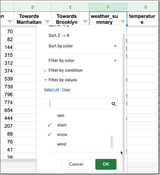
Click on the filter on the weather_summary column to open the filter menu.
Click “Clear” to deselect all the items.
Then choose “sleet” and “snow” as your filter values.
Hit OK to implement the filter.
You end up with 61 rows of data showing only the “sleet” or “snow” rows.
Now let’s see that same filter in BigQuery.
Step 12: WHERE filter keyword
Add the WHERE clause after the FROM line, and use the OR statement to filter on two conditions.
SELECT
  *
FROM
  `start-bigquery-294922.start_bigquery.brooklyn_bridge_pedestrians`
WHERE
  weather_summary = 'snow' OR weather_summary = 'sleet'
Check the count of the rows outputted by the this query. It’s 61, which matches the row count from your Google Sheet.
Ordering Data
Another common operation we want to do to understand our data is sort it. In Sheets we can either sort through the filter menu options or through the Data menu.
Step 13: Sorting data in Google Sheets
Remove the sleet and snow filter you applied above.
On the temperature column, click the Sort A → Z option, to sort the lowest temperature records to the top.
(Quick aside: it’s amazing to still see so many people walking across the bridge in sub-zero temps!)
Let’s recreate this sort in BigQuery.
Step 14: ORDER BY sort keyword
Add the ORDER BY clause to your query, after the FROM clause:
SELECT
  *
FROM
  `start-bigquery-294922.start_bigquery.brooklyn_bridge_pedestrians`
ORDER BY
  temperature ASC;
Use the keyword ASC to sort ascending (A – Z) or the keyword DESC to sort descending (Z – A).
You might notice that the first two records that show up have “null” in the temperature column, which means that no temperature value was recorded for those rows or it’s missing.
Let’s filter them out with the WHERE clause, so you can see how the WHERE and ORDER BY fit together.
Step 15: Filter out null values
The WHERE clause comes after the FROM clause but before the ORDER BY.
Remove the nulls by using the keyword phrase “IS NOT NULL”.
SELECT
  *
FROM
  `start-bigquery-294922.start_bigquery.brooklyn_bridge_pedestrians`
WHERE
  temperature IS NOT NULL
ORDER BY
  temperature ASC;
Aggregating Data
In Google Sheets, we group data with a pivot table.
Typically you choose a category for the rows and aggregate (summarize) the data into each category.
In this dataset, we have a row of data for each hour of each day. We want to group all 24 rows into a single summary row for each day.
Step 16: Pivot tables in Google Sheets
With your cursor somewhere in the pedestrian dataset, click Data < Pivot table
In the pivot table, add hour_beginning to the Rows.
Uncheck the “Show totals” checkbox.
Right click on one of the dates in the pivot table and choose “Create pivot date group“.
Select “Day of the month” from the list of options.
Add hour_beginning to Rows again, and move it so it’s the top category in Rows.
Check the “Repeat row labels” checkbox.
Right click on one of the dates in the pivot table and choose “Year-Month” from the list of options.
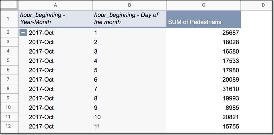
Add Pedestrians field to the Values section, and leave it set to the default SUM.
Your pivot table should look like this, with the total pedestrian counts for each day:
Now let’s recreate this in BigQuery.
If you’ve ever used the QUERY function in Google Sheets then you’re probably familiar with the GROUP BY keyword. It does exactly what the pivot table in Sheets does and “rolls up” the data into the summary categories.
Step 17: GROUP BY in BigQuery to aggregate data
First off, you need to use the EXTRACT function to extract the date from the timestamp in BigQuery.
This query selects the extracted date and the original timestamp, so you can see them side-by-side:
SELECT
  EXTRACT(DATE FROM hour_beginning) AS bb_date,
  hour_beginning
FROM
  `start-bigquery-294922.start_bigquery.brooklyn_bridge_pedestrians`
The EXTRACT DATE function turns “2017-10-01 00:00:00 UTC” into “2017-10-01”, which lets us aggregate by the date.
Modify the query above to add the SUM(Pedestrians) column, remove the “hour_beginning” column you no longer need and add the GROUP BY clause, referencing the grouping column by the alias name you gave it “bb_date”
SELECT
  EXTRACT(DATE FROM hour_beginning) AS bb_date,
  SUM(Pedestrians) AS bb_pedestrians
FROM
  `start-bigquery-294922.start_bigquery.brooklyn_bridge_pedestrians`
GROUP BY
  bb_date
The output of this query will be a table that matches the data in your pivot table in Google Sheet. Great work!
Functions in BigQuery
You’ll notice we used a special function (EXTRACT) in that previous query.
Like Google Sheets, BigQuery has a huge library of built-in functions. As you make progress on your BigQuery journey, you’ll find more and more of these functions to use.
For more information on functions in BigQuery, have a look at the function reference.
We saw the WHERE clause earlier, which lets you filter rows in your dataset.
However, if you aggregate your data with a GROUP BY clause and you want to filter this grouped data, you need to use the HAVING keyword.
Remember:
WHERE = filter original rows of data in dataset
HAVING = filter aggregated data after a GROUP BY operation
To conceptualize this, let’s apply the filter to our aggregate data in the Google Sheet pivot table.
Step 18: Pivot table filter in Google Sheets
Add hour_beginning to the filter section of your pivot table in Google Sheets.
Filter by condition and set it to Date is before > exact date > 11/01/2017
This filter removes rows of data in your Pivot Table where the data is on or after 1 November 2017. It leaves just the October 2017 data.
By now, I think you know what’s coming next.
Let’s apply that same filter condition in BigQuery using the HAVING keyword.
Step 19: HAVING filter keyword
Add the HAVING clause to your existing query, to filter out data on or after 1 November 2017.
Only data that satisfies the HAVING condition (less than 2017-11-01) is included.
SELECT
  EXTRACT(DATE FROM hour_beginning) AS bb_date,
  SUM(Pedestrians) AS bb_pedestrians
FROM
  `start-bigquery-294922.start_bigquery.brooklyn_bridge_pedestrians`
GROUP BY
  bb_date
HAVING
  bb_date < '2017-11-01'
The output of this query is 31 rows of data, for each day of the month of October.
Get started with Google BigQuery: Joining Data
A SQL Query walks into a bar.
In one corner of the bar are two tables.
The Query walks up to the tables and asks:
Mind if I join you?
JOIN pulls multiple tables together, like the VLOOKUP function in Google Sheets. Let's start in your Google Sheet.
Step 20: Vlookup to join data tables in Google Sheets
Create a new blank Sheet inside your Google Sheet.
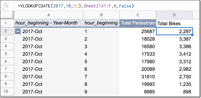
Drag the formula down the rows to complete the dataset.
The data in your Sheet now looks like this:
That's great!
We summarized the pedestrian data by day and joined the bicycle data to it, so you can compare the two numbers.
As you can see, there's around 10k - 20k pedestrian crossings/day and about 2k - 3k bike crossings/day.
Joining tables in BigQuery
Let's recreate this table in BigQuery, using a JOIN.
Step 21: Upload bicycle data to BigQuery
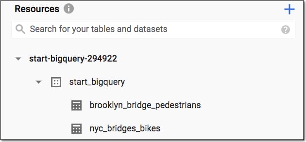
Following step 5 above, create a new table in your start_bigquery dataset and upload the second dataset, of bike data for NYC bridges from October 2017.
Name your table "nyc_bridges_bikes"
Your project should now look like this in the Resources pane in the left sidebar:
What we want to do now is take the table the you created above, with pedestrian data per day, and add the bike counts for each day to it.
To do that we use an INNER JOIN.
There are several different types of JOIN available in SQL, but we'll only look at the INNER JOIN in this article. It creates a new table with only the rows from each of the constituent tables that meet the join condition.
In our case the join condition is matching dates from the pedestrian table and the bike table.
We'll end up with a table consisting of the date, the pedestrian data and the bike data.
Ready? Let's go.
Step 22: JOIN the datasets in BigQuery
First, wrap the query you wrote above with the WITH clause, so you can refer to the temporary table that's created by the name "pedestrian_table".
WITH pedestrian_table AS (
  SELECT
    EXTRACT(DATE FROM hour_beginning) AS bb_date,
    SUM(Pedestrians) AS bb_pedestrians
  FROM
    `start-bigquery-294922.start_bigquery.brooklyn_bridge_pedestrians`
  GROUP BY
    bb_date
  HAVING
    bb_date < '2017-11-01'
)
Next, select both columns from the pedestrian table and one column from the bike table:
SELECT
  pedestrian_table.bb_date,
  pedestrian_table.bb_pedestrians,
  bike_table.Brooklyn_Bridge AS bb_bikes
FROM
  pedestrian_table
Of course, you need to add in the bike table to the query so the bike data can be retrieved:
INNER JOIN
  `start-bigquery-294922.start_bigquery.nyc_bridges_bikes` AS bike_table
Finally, specify the join condition, which tells the query what columns to match:
ON
  pedestrian_table.bb_date = bike_table.Date
Phew, that's a lot!
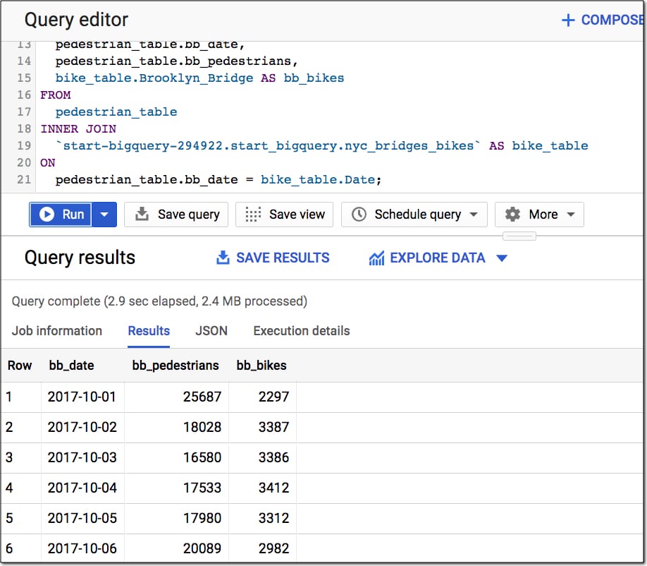
Here's the full query:
WITH pedestrian_table AS (
  SELECT
    EXTRACT(DATE FROM hour_beginning) AS bb_date,
    SUM(Pedestrians) AS bb_pedestrians
  FROM
    `start-bigquery-294922.start_bigquery.brooklyn_bridge_pedestrians`
  GROUP BY
    bb_date
  HAVING
    bb_date < '2017-11-01'
)
SELECT
  pedestrian_table.bb_date,
  pedestrian_table.bb_pedestrians,
  bike_table.Brooklyn_Bridge AS bb_bikes
FROM
  pedestrian_table
INNER JOIN
  `start-bigquery-294922.start_bigquery.nyc_bridges_bikes` AS bike_table
ON
  pedestrian_table.bb_date = bike_table.Date
You'll notice that the names of the columns in our SELECT clause are preceded by the table name, e.g. "pedestrian_table.bb_date".
This ensures there is no confusion over which columns from which tables are being requested. It’s also necessary when you join tables that have common column headings.
The output of this query is the same as the table you created in your Google Sheet step 20 (using the pivot table and VLOOKUP).
Formatting Your Queries
Last couple of things to mention with the SQL syntax is how to add comments and format your queries.
Step 23: Formatting Your Queries
You can add comments in SQL two ways, with a double dash "--" or forward slash and star combination "/*...*/".
-- single line comment, ignored when the program is run
or
/* multi-line comment
everything between the slash-stars
is ignored by the program when it's run */
It's also a good habit to put SQL keywords on separate lines, to make it more readable.
Use the menu More > Format to do this automatically.
Section 5: Export Data Out Of BigQuery
You have a few options to export data out of BigQuery.
In the Query results section of the editor, click on the "SAVE RESULTS" button to:
Save as a CSV file
Save as a JSON file
Export query results to Google Sheets (up to 16,000 rows)
Copy to Clipboard
In this tutorial, we're going to export the data out of BigQuery and back into a Google Sheet, to create a chart. We're able to do this because the summary dataset we've created is small (it's aggregated data we want to use to create a chart, not the row-by-row data).
Explore BigQuery Data in Sheets or Data Studio
If you want to create a chart based on hundreds of thousands or millions of rows of data, then you can explore the data in Google Sheets or Data Studio directly, without taking it out of BigQuery.
Click on the "EXPLORE DATA" option in the Query results section of the editor:
Explore in Google Sheets using Connected Sheets (Enterprise customers only)
Explore directly in Data Studio
Get started with Google BigQuery: Export to Google Sheets
In this tutorial, the output table is easily small enough to fit in Google Sheets, so let's export the data out of BigQuery and into Sheets.
There, we'll create chart a chart showing the pedestrian and bike traffic across the Brooklyn Bridge.
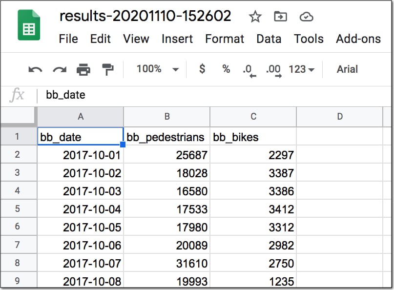
Step 24: Export Data Out Of BigQuery
Run your query from step 22 above, which outputs a table with date, pedestrian count and bike count.
Click on the "SAVE RESULTS" and select Google Sheets.
Hit Save.
Select Open in the toast popup that tells you a new Sheet has been created, or find it in your Drive root folder (the top folder).
The data now looks like this in the new Sheet:
Yay! Back on familiar territory!
From here, you can do whatever you want with your data.
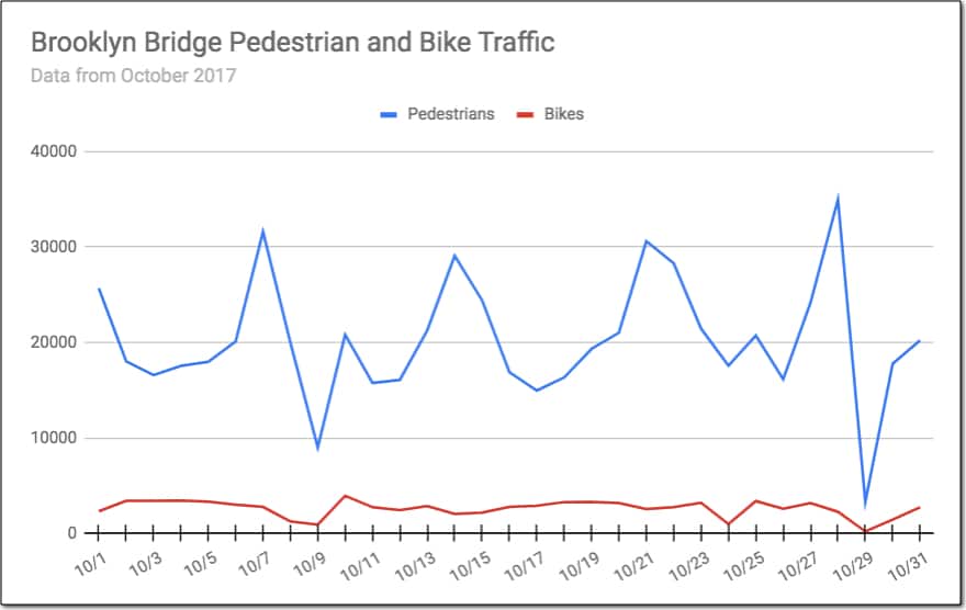
I chose to create a simple line chart to compare the daily foot and bike traffic across Brooklyn Bridge:
Step 25: Display the data in a chart in Google Sheets
Highlight your dataset and go to Insert > Chart
Select the line chart (if it isn't selected as the default).
Fix the title and change the column names to display better in chart.
Under the Horizontal Axis option, check the "Treat labels as text" checkbox.
See how much information this chart gives you, compared to thousands of rows of raw data.
It tells you the story of the pedestrian and bike traffic crossing the Brooklyn Bridge.
Congratulations!
You've completed your first end-to-end BigQuery + Google Sheets data analysis project.
You’ve decided you want to be a freelance Google Sheets developer. Great!
But how do you get started?
I get asked this question a lot, so I’ve compiled my email answers into this blog post.
But first, let me share my story, so you hear it from the horse’s mouth:
My Journey As A Freelance Google Sheets Developer
I quit my corporate accounting job in late 2014. I was unhappy because I felt like I was living someone else’s life. Deep down, I knew I wanted to do something technical and creative.
After leaving corporate accounting, I spent six months learning to code and looking for tech roles.
Following the advice for job hunters at the time, I created a blog (this website) and began writing about about lots of different technical topics including coding, data and Google Sheets. Without planning it, I was learning in public.
And it led to my first client, which was fortunate because I wasn’t getting anywhere applying for tech roles. (And I really mean that, I applied for a bunch of web developer roles and data analyst roles and was yet to get past the first interview. Things worked out in the end though.)
First Client
My first client was a small real estate company using Forms and Sheets to collect data from their sales agents. They’d seen the dashboard tutorial on my website and asked me to create something similar for them.
I charged them $400 and the project took around 10 hours. (Actually, it could well have been 20 hours because I didn’t track my time when I first started.)
Although the dashboard was basic, it delivered huge value to the client.
Cultivating Inbound Leads
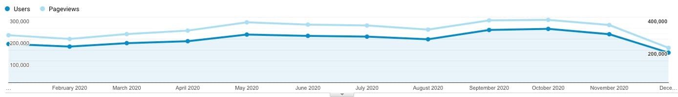
I kept publishing content about Google Sheets and Apps Script. The website picked up more search traffic through 2015 and each subsequent year since.
I realize I was lucky with my timing since Google Sheets growth was exploding and there weren’t many resources online.
The search traffic brought more inbound leads: people contacting me for help with their projects.
Once you have a reliable source of leads coming into your business, you can focus on being more efficient and expanding beyond the feast to famine freelance cycle.
After a few years of freelancing, I stopped trading time for money (which we discuss below) and eventually moved to creating online courses and teaching online (but that’s a story for another day).
Yeah, this is a 100% truthful representation of the freelancer life ?
Your journey won’t look like mine, but there are universal actions you can take to get there quicker than I did. So, turning our attention back to you, here are some actionable steps you can take today to start your freelancer journey:
Freelance Google Sheets Developer Playbook
This short guide is broken into a few sections dealing with different aspects of freelancing.
The most important lesson to takeaway is that you need to spend as much, if not more, time on sales as on the hard, technical skills.
With that in mind, let’s begin with the most important thing you can do for your freelance career: get clients!
1. How To Get Clients As A Freelance Google Sheets Developer
This is the most important thing you do.
Not your Google Sheets skills. Not your business skills. Not time management. No, the most important thing is getting clients. (And then making them happy of course.)
This will determine whether or not you succeed, so focus heavily on this from day one.
Specifically, here are some ideas to get your first clients:
Email all your friends/family/contacts to tell them you’re doing this and ask for work referrals.
Offer to do pro-bono (free) spreadsheet work for small orgs/non-profits to gain some experience and testimonials.
Look for freelance spreadsheet work on sites like Upwork and Fiverr. Choose one and build a portfolio/reputation there.
Look for Google Sheet jobs on job sites like Indeed (hard to find ones where this is the main skill required though).
Keep your eyes on “spreadsheet” companies that build solutions on top of Google Sheets (e.g. this list on Product Hunt). They occasionally hire part-time and full-time spreadsheet developers.
Create a (simple) website and share your work/ideas/knowledge. This will help you figure out what you want to do and demonstrate you can do it.
Add a “Hire Me” page with details of your work and testimonials. Make it easy for someone to contact you through a form.
Create a white-paper or short ebook that’s helpful in your industry and share it with your network. Ask them to share with their networks. You’d be amazed at how shareable a high-value asset like an ebook can be. Creating content is a high leverage activity (i.e. the reward > the effort, at least over the long run).
2. Fees: What To Charge As A Freelance Google Sheets Developer?
“What should I charge?” is probably the second most frequently asked question (after “how do I get clients?”).
The answers and advice are across the board:
“Do it for free to get exposure.” (But how will you pay the bills?)
“Charge what you’re worth.” (Super helpful when you’re starting out!)
“Whatever number you have in your head, double it.” (Ok, that’s not bad advice as most freelancers undercharge).
Consider Both Sides
Most of us, especially when we’re new to this game, think about fees based on what it takes to complete the project, i.e. how many hours it will take.
Maybe it’ll take me 15 hours, which, at $100 / hour, is $1,500. Bingo! Invoice for $1,500.
That’s fine, but it’s only one way to think about it.
The other way is to think, “what’s the value of this to the client?”
Suppose they’ve asked you to automate their reporting pipeline and they’ll save 3 hours a week. Now that analyst’s time can be repurposed to do more meaningful work.
From the client’s perspective, this is hugely valuable.
They’d probably happily pay multiples of $1,500 for that solution.
So you have to think about both angles: your side, in terms of how much time it’ll take you to do the project, and then from the client’s side, and what’s the value there.
Hourly Pricing
The rate is dependent on many factors: your experience, the niche you’re working in, the market you operate in etc.
Just remember, you’re competing with people who answer questions for free in forums and folks who charge $5/hr on Upwork.
It’s hard to compete on price and you can’t work for $5/hr if you’re living in the U.S.
Assuming equal spreadsheet skills, you can differentiate yourself by being super reliable, a pleasure to work with, a great communicator, knowledgeable about the client’s industry, etc.
And then you can consider consulting rates for Google Sheets work in the range of $50/hr – $150/hr.
Project Pricing
As you improve your systems and grow your business, you’ll become more efficient at solving problems (for example, you have templates for contracts, NDAs, etc. or a gallery of solutions that you can partially re-use).
It makes sense to ditch hourly rates and move to project rates. This way, your efficiency is rewarded. If you do project pricing though, you have to define the scope of work carefully and precisely, to avoid scope creep.
For example, rather than say “Includes planning calls” in your scope, say “includes two 30-minute planning calls” so you set expectations with the client. They won’t ask for more and neither party will expect anything different.
Most Google Sheets development projects will be one-off, but you may get lucky and land a client on a monthly retainer basis, where you’re paid to keep their Google Sheets humming along each month.
Think about the “both sides” idea discussed above. Work out the hours you think it’ll take and use that as your lower pricing bound. Then think about the value to the client and come up with an upper bound. Pitch the client with your bid somewhere between these two bounds.
Pricing Strategy Tips
You might start with a few small free projects to generate leads and portfolio pieces.
Then start charging an hourly rate on the lower end, say $40/hour.
Raise your rates every 6 months or so early on, until you find the optimum level that keeps you busy and maximises your earnings.
Once you have some experience under your belt, try project pricing so your efficiency is rewarded.
Push yourself to pitch higher than you’re comfortable with. If the client rejects your offer you can always go back with a lower offer.
When you propose your opening bid, price it high enough that you have wiggle room. The client may counter with their offer and if you’ve priced low to begin with, you won’t have room to go down.
3. How To Be A Good Freelance Google Sheets Developer
Once you’ve got your first client, you want to make them happy. Happy clients return for more work and refer you to their network.
Follow these few simple steps and you’ll be way ahead of your competition:
Always be polite and courteous in your communications. If you feel like emotion is clouding your decision, walk away from the email or say “I’ll get back to you” and sleep on it. Inevitably, when the fog lifts, you can see the correct decision.
Always be professional and do what you say you’re going to do.
Stick to deadlines and be on time with your submissions. (If you can’t hit a deadline, let the client know as soon as possible and they’ll generally be understanding.)
Be honest with your clients, e.g. if you need more time, it’s going to cost more.
Have a bias towards over-communicating rather than under-communicating. Clients appreciate being kept in the loop.
Have a bias towards action and don’t expect to get everything right first time.
Remember, you’re serving the client, not the other way around. Focus on delivering value to the client, not treating them like an ATM.
4. Implement Systems To Increase Efficiency
Set up systems as soon as you can. It’ll be hugely beneficial for you.
Pre Engagement Phase
The pre-client phase is one area where it’s easy to lose a lot of time. (I’m speaking from experience.) It’s a great area to implement systems to save yourself time and headaches. For example, consider:
Using a service like Calendly to schedule calls, rather than back and forth emails.
Creating a standard work template and pricing structure so you can easily see whether clients are a good fit.
Setting a minimum project price and let potential clients know relatively early in the process, so you don’t waste time with people who won’t pay you.
Set up a robust Customer Relationship Management (CRM) workflow (doesn’t have to be an expensive tool, a Google Sheet also works). Whenever clients dry up, you can email former clients to see if they need help.
During the Project
Use a time tracking system (e.g. Toggl) to track your time. This will be super helpful for costing out future projects as well as the current one.
Batch your time so you avoid too much context switching. For example, schedule all calls on Tuesday afternoons. Open and reply to emails twice a day in 30-minute blocks, then keep your email shut in between (not always possible).
After the Project
Create a standard post-engagement workflow. You have the opportunity to leave the client feeling happy and help your future business prospects.
Check the client is happy and whether there’s anything else you can do for them.
Systemize your payment process to make sure you get paid in a timely fashion. I use Harvest App to create and send invoices.
Ask for testimonials. Use a Google Form so they’re all together in a Google Sheet and you can access them anytime.
5. Niche Down By Industry
Focussing on a specific industry has many benefits:
You develop industry knowledge, which improves the quality of your work product.
You develop a reputation as an expert in the field, the “go-to” person for this type of work.
You develop a network and get referrals.
You can more easily systemize your business e.g. client onboarding.
You can even productize your work e.g. create a Google Sheets template for that industry. This is great for lead generation and could potentially be a revenue generator.
Don’t stress too much about a niche to focus on when you’re just getting started though, unless you have prior experience that gives you a clear advantage.
Otherwise, see what type of work you like doing and what’s popular with your clients. I did Excel, SQL and Tableau consulting and training, as well as Google Sheets work, for the first 2 years, before really doubling down on just Google products. And I worked across all industries to begin with.
Many small businesses, nonprofits and mom-and-pop stores could use help with their data, which in all likelihood exists in spreadsheets!
6. Scale
Finding clients and doing high quality work will always be the two most important aspects of your business.
As you scale, you grow from the feast-to-famine freelancer model to a more predictable monthly take-home as a small business.
You’ll need to systemize more parts of the business so you can focus less of your time on repeatable tasks (like invoicing) and more time on high-value, unique tasks like finding new clients and hiring staff members.
Freelancer To Business Journey
Freelance Google Sheets developer → sole-member business → sole-member business with an assistant → sole-member business with contractors → agency business model with full-time people
At some point you need to decide if you want to do the work or run the business. You can’t do both.
I love my work, so I’ve deliberately kept myself as a single-member LLC with one assistant, so I can keep doing the work.
But it’s an equally valid path to hire contractors, and eventually employees, who carry out the actual spreadsheet work, whilst you run and scale the business.
Some ideas to think about:
Find other contractors with complimentary skills so you can refer work to each other, or collaborate together on projects.
Outsource non-core tasks. For example, hire a bookkeeper to do your accounting for you.
Get rid of clients that are hard work (because they pay low rates, haggle over everything, don’t respond to you etc.). Marie Kondo your client list! Does this client bring me joy? If not, let them go!
Culture also becomes a critical part of your success as you start to hire people.
It’s simple in theory but hard to execute: hire great people, give them a compelling vision for the business and get out of their way so they can do great work.