In this post, I’m going to show you how to create radial bar charts in Google Sheets.
They look great and grab your attention, which is important in this era of information overload.
But they should be used sparingly because they’re harder to read than a regular bar chart (because it’s harder to compare the length of the curved bars).
How To Create A Radial Bar Chart In Google Sheets
Let’s begin with the data.
In this example, we’ll create a radial bar chart in Google Sheets with 3 series.
We need a column of values for these 3 series, for example, products with a number of units sold.
Next, we need some upper limit (max value) for our bars. This allows us to scale the bars properly.
Lastly, we need a helper column that calculates the difference between the max value and the actual value.
Here’s the data for the radial bar chart, in cells E3:H6:
Ok, I’m going to let you in on a little secret now…
This is not a single chart. No sir, it’s three charts overlaid on top of each other.
And yes, this means it takes three times as long to create!
Step 1: Create the inner circle
Highlight the first row of data but exclude the max value column. In the example dataset above, highlight E4:G4 and insert a chart.
Select a doughnut chart.
Under the Setup menu, make sure to check the “Switch rows/columns” checkbox, so your chart looks like this:
Under the customize menu of the chart tool, set the following conditions:
Background color: None
Chart border color: None
Donut hole size: 67%
Set Slice 2 color to none
Remove the chart title
Set the legend to none
This is what the inner donut should look like:
Step 2: Create the middle circle
Repeat the steps above for the inner circle, but use the next row of data, choose a different color, and set the donut hole size to 77% (you may have to experiment with these percentages to line everything up at the end).
Drag the second donut chart on top of the first and line up the radial bars to get:
Step 3: Create the outer circle
Again, repeat the steps above from the inner circle to create a third donut chart, using the third row of data, a different color, and setting the donut hole size to 81% (again, this might need tweaking to line everything up).
Drag this third donut chart on top of the other two and you have a radial bar chart in Google Sheets!
Note on editing charts:
Since the charts are placed on top of each other, you’ll only be able to access the top chart to edit. You’ll have to move it to the side to access the chart underneath, and then move that one if you want to access the inner chart.
Step 4: Add the data labels
It gets messy to add the data labels to each chart through the chart editor, so I opted to create formulas to add my data labels into the cells next to each bar of the radial bar chart.
To access cells underneath the charts, click on a cell outside of the chart area and then use the arrow keys on your keyboard to reach the desired cell.
My friend Jeff Sauer, who founded Data Driven U to teach people data-driven marketing, contacted me recently about creating a radial bar chart for one of his workshops.
He is graciously sharing his report here, so you can see a radial bar chart with six rings:
This is a screenshot of his Google Sheet!
(If you’re looking for top draw digital marketing, then you should definitely check out Jeff’s site: DataDrivenU.com This is not an affiliate link, just a personal recommendation!)
You’ve probably also seen a radial bar chart in the wild with the Apple Watch Rings Chart!
This tutorial is written for Google Sheets users who have datasets that are too big or too slow to use in Google Sheets. It’s written to help you get started with Google BigQuery.
If you’re experiencing slow Google Sheets that no amount of clever tricks will fix, or you work with datasets that are outgrowing the 10 million cell limit of Google Sheets, then you need to think about moving your data into a database.
As a Google user, probably the best and most logical next step is to get started with Google BigQuery and move your data out of Google Sheets and into BigQuery.
By the end of this tutorial, you will have created a BigQuery account, uploaded a dataset from Google Sheets, written some queries to analyze the data and exported the results back to Google Sheets to create a chart.
You’ll also do the same analysis side-by-side in a Google Sheet, so you can understand exactly what’s happening in BigQuery.
I’ve highlighted the action steps throughout the tutorial, to make it super easy for you to follow along:
Google BigQuery exercise steps are shown in blue.
Actions for you to do in Google BigQuery.
Google Sheet exercise steps are shown in green.
Actions for you to do in Google Sheets.
Section 1: What is BigQuery?
Google BigQuery is a data warehouse for storing and analyzing huge amounts of data.
Officially, BigQuery is a serverless, highly-scalable, and cost-effective cloud data warehouse with an in-memory BI Engine and machine learning built in.
This is a formal way of saying that it’s:
Works with any size data (thousands, millions, billions of rows…)
Easy to set up because Google handles the infrastructure
Grows as your data grows
Good value for money, with a generous free tier and pay-as-you-go beyond that
Lightning fast
Seamlessly integrated with other Google tools, like Sheets and Data Studio
Can import and export data from and to many sources
Has Built-in machine learning, so predictive modeling can be set up quickly
What’s the difference between BigQuery and a “regular” database?
BigQuery is a database optimized for storing and analyzing data, not for updating or deleting data.
It’s ideal for data that’s generated by e-commerce, operations, digital marketing, engineering sensors etc. Basically, transactional data that you want to analyze to gain insights.
A regular database is suitable for data that is stored, but also updated or deleted. Think of your social media profile or customer database. Names, emails, addresses, etc. are stored in a relational database. They frequently need to be updated as details change.
Section 2: Google BigQuery Setup
It’s super easy to get started wit Google BigQuery!
There are two ways to get started: 1) use the free sandbox account (no billing details required), or 2) use the free tier (requires you to enter billing details, but you’ll also get $300 free Cloud credits).
In either case, this tutorial won’t cost you anything in BigQuery, since the volume of data is so tiny.
We’ll proceed using the sandbox account, so that you don’t have to enter any billing details.
A new project called “My First Project” is automatically created
In the left side pane, scroll down until you see BigQuery and click it
Here’s that process shown as a GIF:
You’re ready for Step 2 below.
BigQuery Console
(click to enlarge)
Here’s what you can see in the console:
The SANDBOX tag to tell you you’re in the sandbox environment
Message to upgrade to the free trial and $300 credit (may or may not show)
UPGRADE button to upgrade out of the Sandbox account
ACTIVATE button to claim the free $300 credit
The current project and where to create new projects
The Query editor window where you type your SQL code
Current project resource
Button to create a new dataset for this project (see below)
Query outputs and table information window
What is the free Sandbox Account?
The sandbox account is an option that lets you use BigQuery without having to enter any credit card information. There are limits to what you can do, but it gives you peace of mind that you won’t run up any charges whilst you’re learning.
In the sandbox account:
Tables or views last 60 days
You get 10 Gb of storage per month for free
And 1 Tb data processing each month
It’s more than enough to do everything in this tutorial today.
Unlike Google Sheets, you have to pay to use BigQuery based on your storage and processing needs.
However, there is a sandbox account for free experimentation (see below) and then a generous free tier to continue using BigQuery.
In fact, if you’re working with datasets that are only just too big for Sheets, it’ll probably be free to use BigQuery or very cheap.
BigQuery charges for data storage, streaming inserts, and for querying data, but loading and exporting data are free of charge.
Your first 1 TB (1,000 GB) per month is free.
Full BigQuery pricing information can be found here.
Clicking on the blue “Try BigQuery free” button on the BigQuery homepage will let you register your account with billing details and claim the free $300 cloud credits.
Section 3: How to get your data into BigQuery
Extracting, loading and transforming (ELT) is sometimes the most challenging and time consuming part of a data analysis project. It’s the most engineering-heavy stage, where the heavy lifting happens.
You can load data into BigQuery in a number of ways:
From a readable data source (such as your local machine)
From Google Sheets
From other Google services, such as Google Ad Manager and Google Ads
Use a third-party data integration tool, e.g. Supermetrics, Stitch
You might want to make a SECOND copy in your Drive folder too, so you can keep one copy untouched for the upload to BigQuery and use the second copy for doing the follow-along analysis in Google Sheets.
The first dataset is a record of pedestrian traffic crossing Brooklyn Bridge in New York city (source).
It’s only 7,000 rows, so it could be easily analyzed in Sheets of course, but we’ll use it here so that you can do the same steps in BigQuery and in Sheets.
The second dataset is a daily total of bike counts for New York’s East River bridges (source).
There’s nothing inherently wrong with putting “small” data into BigQuery. Yes, it’s designed for truly gigantic datasets (billions of rows+) but it works equally well on data of any size.
Back in the BigQuery Console, you need to set up a project before you can add data to it.
Get started with Google BigQuery: Loading data From A Google Sheet
Think of the Project as a folder in Google Drive, the Dataset as a Google Sheet and the Table as individual Sheet within that Google Sheet.
The first step to get started with Google BigQuery is to create a project.
In step 1, BigQuery will have automatically generated a new project for you, called “My First Project”.
If it didn’t, or you want to create another new project, here’s how.
Step 3: Create a new Project
In the top bar, to the right of where it says “Google Cloud Platform”, click on Project drop-down menu.
In the popup window, click NEW PROJECT.
Give it a name, organization (your domain) and location (parent organization or folder).
Optionally, you can choose to bookmark this project in the Resources section of the sidebar. Click “PIN PROJECT” to do this.
Step 4: Create a new Dataset
Next you need to create a dataset by clicking “CREATE DATASET“.
Name it “start_bigquery”. You’re not allowed to have any spaces or special characters apart from the underscore.
Set the data location to your locale, leave the other settings alone and then click “Create dataset”
This new dataset will show up underneath your project name in the sidebar.
Step 5: Create a new Table
With the dataset selected, click on the “+ CREATE TABLE” or big blue plus button.
You want to select “Drive”, add the URL and set the file format to Google Sheets.
Name your table “brooklyn_bridge_pedestrians”.
Choose Auto detect schema.
Under Advanced settings, tell BigQuery you have a single header row to skip by entering the value 1.
Your settings should look like this:
If you make a mistake, you can simply delete the table and start again.
Section 4: Analyzing Data in BigQuery
Google BigQuery uses Structure Query Language (SQL) to analyze data.
The Google Sheets Query function uses a similar SQL style syntax to parse data. So if you know how to use the Query function then you basically know enough SQL to get started with Google BigQuery!
Basic SQL Syntax for BigQuery
The basic SQL syntax to write queries looks like this:
SELECT these columns
FROM this table
WHERE these filter conditions are true
GROUP BY these aggregate conditions
HAVING these filters on aggregates
ORDER BY i.e. sort by these columns
LIMIT restrict answer to X number of rows
You’ll see all of these keywords and more in the exercises below.
Get started with Google BigQuery: First Query
The BigQuery console provides a button that gives you a starter query.
Step 6: Write your first query
Click on “QUERY TABLE” and this query shows up in your editor window:
SELECT FROM `start-bigquery-294922.start_bigquery.brooklyn_bridge_pedestrians` LIMIT 1000
Modify it by adding a * between the SELECT and FROM, and reducing the number after LIMIT to 10:
SELECT
  *
FROM
  `start-bigquery-294922.start_bigquery.brooklyn_bridge_pedestrians`
LIMIT
  10
Then format your query across multiple lines with through the menu: More > Format
SELECT
*
FROM
`start-bigquery-294922.start_bigquery.brooklyn_bridge_pedestrians`
LIMIT
10
Click “▶️ Run” to execute the query.
The output of this query will be 10 rows of data showing under the query editor:
(click to enlarge)
Woohoo!
You just wrote your first query in Google BigQuery.
Let’s continue and analyze the dataset:
Exercise 2: Analyzing Data In BigQuery
Run through the following steps:
Step 7: tell the story of one row
I always advocate doing this with any new dataset.
Write a query that selects all the columns (SELECT *) and a limited number of rows (e.g. LIMIT 10), as you did in step 6 above.
Run that query and look at the output. Scan across one whole row. Look at every column and think about what data is stored there.
Think about doing the equivalent step in Google Sheets. Look at your dataset and scroll to the right, telling the story of a single row.
We do this step to understand our data, before getting too immersed in the weeds.
Select Specific Columns
Step 8: Select specific columns
Select specific columns by writing the column names into your query.
You can also click on column names in the schema view (click on the table name in the left sidebar to access this) to add them to the query directly.
SELECT
  hour_beginning,
  location,
  Pedestrians,
  weather_summary
FROM
  `start-bigquery-294922.start_bigquery.brooklyn_bridge_pedestrians`
LIMIT
  10
Math Operations
Let’s find out the total number of pedestrians that crossed the Brooklyn Bridge across the whole time period.
Step 9: Calculate total in Google Sheets
Open the Google Sheet you copied in Step 2, called “Copy of Brooklyn Bridge pedestrian count dataset”
Add this simple SUM function to cell C7298 to calculate the total:
=SUM(C2:C7297)
This gives an answer of 5,021,692
Let’s see how to do that in BigQuery:
Step 10: Math operations in BigQuery
Write a query with the pedestrians column and wrap it with a SUM function:
SELECT
  SUM(Pedestrians) AS total_pedestrians
FROM
  `start-bigquery-294922.start_bigquery.brooklyn_bridge_pedestrians`
This gives the same answer of 5,021,692
You’ll notice that I gave the output a new column name using the code “AS total_pedestrians“. This is similar to using the LABEL clause in the QUERY function in Google Sheets
Filtering Data
In SQL, the WHERE clause is used to filter rows of data.
It acts in the same way as the filter operation on a dataset in Google Sheets.
Step 11: Filtering data in Google Sheets
Back in your Google Sheet with the pedestrian data, add a filter to the dataset: Data > Create a filter
Click on the filter on the weather_summary column to open the filter menu.
Click “Clear” to deselect all the items.
Then choose “sleet” and “snow” as your filter values.
Hit OK to implement the filter.
You end up with 61 rows of data showing only the “sleet” or “snow” rows.
Now let’s see that same filter in BigQuery.
Step 12: WHERE filter keyword
Add the WHERE clause after the FROM line, and use the OR statement to filter on two conditions.
SELECT
  *
FROM
  `start-bigquery-294922.start_bigquery.brooklyn_bridge_pedestrians`
WHERE
  weather_summary = 'snow' OR weather_summary = 'sleet'
Check the count of the rows outputted by the this query. It’s 61, which matches the row count from your Google Sheet.
Ordering Data
Another common operation we want to do to understand our data is sort it. In Sheets we can either sort through the filter menu options or through the Data menu.
Step 13: Sorting data in Google Sheets
Remove the sleet and snow filter you applied above.
On the temperature column, click the Sort A → Z option, to sort the lowest temperature records to the top.
(Quick aside: it’s amazing to still see so many people walking across the bridge in sub-zero temps!)
Let’s recreate this sort in BigQuery.
Step 14: ORDER BY sort keyword
Add the ORDER BY clause to your query, after the FROM clause:
SELECT
  *
FROM
  `start-bigquery-294922.start_bigquery.brooklyn_bridge_pedestrians`
ORDER BY
  temperature ASC;
Use the keyword ASC to sort ascending (A – Z) or the keyword DESC to sort descending (Z – A).
You might notice that the first two records that show up have “null” in the temperature column, which means that no temperature value was recorded for those rows or it’s missing.
Let’s filter them out with the WHERE clause, so you can see how the WHERE and ORDER BY fit together.
Step 15: Filter out null values
The WHERE clause comes after the FROM clause but before the ORDER BY.
Remove the nulls by using the keyword phrase “IS NOT NULL”.
SELECT
  *
FROM
  `start-bigquery-294922.start_bigquery.brooklyn_bridge_pedestrians`
WHERE
  temperature IS NOT NULL
ORDER BY
  temperature ASC;
Aggregating Data
In Google Sheets, we group data with a pivot table.
Typically you choose a category for the rows and aggregate (summarize) the data into each category.
In this dataset, we have a row of data for each hour of each day. We want to group all 24 rows into a single summary row for each day.
Step 16: Pivot tables in Google Sheets
With your cursor somewhere in the pedestrian dataset, click Data < Pivot table
In the pivot table, add hour_beginning to the Rows.
Uncheck the “Show totals” checkbox.
Right click on one of the dates in the pivot table and choose “Create pivot date group“.
Select “Day of the month” from the list of options.
Add hour_beginning to Rows again, and move it so it’s the top category in Rows.
Check the “Repeat row labels” checkbox.
Right click on one of the dates in the pivot table and choose “Year-Month” from the list of options.
Add Pedestrians field to the Values section, and leave it set to the default SUM.
Your pivot table should look like this, with the total pedestrian counts for each day:
Now let’s recreate this in BigQuery.
If you’ve ever used the QUERY function in Google Sheets then you’re probably familiar with the GROUP BY keyword. It does exactly what the pivot table in Sheets does and “rolls up” the data into the summary categories.
Step 17: GROUP BY in BigQuery to aggregate data
First off, you need to use the EXTRACT function to extract the date from the timestamp in BigQuery.
This query selects the extracted date and the original timestamp, so you can see them side-by-side:
SELECT
  EXTRACT(DATE FROM hour_beginning) AS bb_date,
  hour_beginning
FROM
  `start-bigquery-294922.start_bigquery.brooklyn_bridge_pedestrians`
The EXTRACT DATE function turns “2017-10-01 00:00:00 UTC” into “2017-10-01”, which lets us aggregate by the date.
Modify the query above to add the SUM(Pedestrians) column, remove the “hour_beginning” column you no longer need and add the GROUP BY clause, referencing the grouping column by the alias name you gave it “bb_date”
SELECT
  EXTRACT(DATE FROM hour_beginning) AS bb_date,
  SUM(Pedestrians) AS bb_pedestrians
FROM
  `start-bigquery-294922.start_bigquery.brooklyn_bridge_pedestrians`
GROUP BY
  bb_date
The output of this query will be a table that matches the data in your pivot table in Google Sheet. Great work!
Functions in BigQuery
You’ll notice we used a special function (EXTRACT) in that previous query.
Like Google Sheets, BigQuery has a huge library of built-in functions. As you make progress on your BigQuery journey, you’ll find more and more of these functions to use.
For more information on functions in BigQuery, have a look at the function reference.
We saw the WHERE clause earlier, which lets you filter rows in your dataset.
However, if you aggregate your data with a GROUP BY clause and you want to filter this grouped data, you need to use the HAVING keyword.
Remember:
WHERE = filter original rows of data in dataset
HAVING = filter aggregated data after a GROUP BY operation
To conceptualize this, let’s apply the filter to our aggregate data in the Google Sheet pivot table.
Step 18: Pivot table filter in Google Sheets
Add hour_beginning to the filter section of your pivot table in Google Sheets.
Filter by condition and set it to Date is before > exact date > 11/01/2017
This filter removes rows of data in your Pivot Table where the data is on or after 1 November 2017. It leaves just the October 2017 data.
By now, I think you know what’s coming next.
Let’s apply that same filter condition in BigQuery using the HAVING keyword.
Step 19: HAVING filter keyword
Add the HAVING clause to your existing query, to filter out data on or after 1 November 2017.
Only data that satisfies the HAVING condition (less than 2017-11-01) is included.
SELECT
  EXTRACT(DATE FROM hour_beginning) AS bb_date,
  SUM(Pedestrians) AS bb_pedestrians
FROM
  `start-bigquery-294922.start_bigquery.brooklyn_bridge_pedestrians`
GROUP BY
  bb_date
HAVING
  bb_date < '2017-11-01'
The output of this query is 31 rows of data, for each day of the month of October.
Get started with Google BigQuery: Joining Data
A SQL Query walks into a bar.
In one corner of the bar are two tables.
The Query walks up to the tables and asks:
Mind if I join you?
JOIN pulls multiple tables together, like the VLOOKUP function in Google Sheets. Let's start in your Google Sheet.
Step 20: Vlookup to join data tables in Google Sheets
Create a new blank Sheet inside your Google Sheet.
Drag the formula down the rows to complete the dataset.
The data in your Sheet now looks like this:
That's great!
We summarized the pedestrian data by day and joined the bicycle data to it, so you can compare the two numbers.
As you can see, there's around 10k - 20k pedestrian crossings/day and about 2k - 3k bike crossings/day.
Joining tables in BigQuery
Let's recreate this table in BigQuery, using a JOIN.
Step 21: Upload bicycle data to BigQuery
Following step 5 above, create a new table in your start_bigquery dataset and upload the second dataset, of bike data for NYC bridges from October 2017.
Name your table "nyc_bridges_bikes"
Your project should now look like this in the Resources pane in the left sidebar:
What we want to do now is take the table the you created above, with pedestrian data per day, and add the bike counts for each day to it.
To do that we use an INNER JOIN.
There are several different types of JOIN available in SQL, but we'll only look at the INNER JOIN in this article. It creates a new table with only the rows from each of the constituent tables that meet the join condition.
In our case the join condition is matching dates from the pedestrian table and the bike table.
We'll end up with a table consisting of the date, the pedestrian data and the bike data.
Ready? Let's go.
Step 22: JOIN the datasets in BigQuery
First, wrap the query you wrote above with the WITH clause, so you can refer to the temporary table that's created by the name "pedestrian_table".
WITH pedestrian_table AS (
  SELECT
    EXTRACT(DATE FROM hour_beginning) AS bb_date,
    SUM(Pedestrians) AS bb_pedestrians
  FROM
    `start-bigquery-294922.start_bigquery.brooklyn_bridge_pedestrians`
  GROUP BY
    bb_date
  HAVING
    bb_date < '2017-11-01'
)
Next, select both columns from the pedestrian table and one column from the bike table:
SELECT
  pedestrian_table.bb_date,
  pedestrian_table.bb_pedestrians,
  bike_table.Brooklyn_Bridge AS bb_bikes
FROM
  pedestrian_table
Of course, you need to add in the bike table to the query so the bike data can be retrieved:
INNER JOIN
  `start-bigquery-294922.start_bigquery.nyc_bridges_bikes` AS bike_table
Finally, specify the join condition, which tells the query what columns to match:
ON
  pedestrian_table.bb_date = bike_table.Date
Phew, that's a lot!
Here's the full query:
WITH pedestrian_table AS (
  SELECT
    EXTRACT(DATE FROM hour_beginning) AS bb_date,
    SUM(Pedestrians) AS bb_pedestrians
  FROM
    `start-bigquery-294922.start_bigquery.brooklyn_bridge_pedestrians`
  GROUP BY
    bb_date
  HAVING
    bb_date < '2017-11-01'
)
SELECT
  pedestrian_table.bb_date,
  pedestrian_table.bb_pedestrians,
  bike_table.Brooklyn_Bridge AS bb_bikes
FROM
  pedestrian_table
INNER JOIN
  `start-bigquery-294922.start_bigquery.nyc_bridges_bikes` AS bike_table
ON
  pedestrian_table.bb_date = bike_table.Date
You'll notice that the names of the columns in our SELECT clause are preceded by the table name, e.g. "pedestrian_table.bb_date".
This ensures there is no confusion over which columns from which tables are being requested. It’s also necessary when you join tables that have common column headings.
The output of this query is the same as the table you created in your Google Sheet step 20 (using the pivot table and VLOOKUP).
Formatting Your Queries
Last couple of things to mention with the SQL syntax is how to add comments and format your queries.
Step 23: Formatting Your Queries
You can add comments in SQL two ways, with a double dash "--" or forward slash and star combination "/*...*/".
-- single line comment, ignored when the program is run
or
/* multi-line comment
everything between the slash-stars
is ignored by the program when it's run */
It's also a good habit to put SQL keywords on separate lines, to make it more readable.
Use the menu More > Format to do this automatically.
Section 5: Export Data Out Of BigQuery
You have a few options to export data out of BigQuery.
In the Query results section of the editor, click on the "SAVE RESULTS" button to:
Save as a CSV file
Save as a JSON file
Export query results to Google Sheets (up to 16,000 rows)
Copy to Clipboard
In this tutorial, we're going to export the data out of BigQuery and back into a Google Sheet, to create a chart. We're able to do this because the summary dataset we've created is small (it's aggregated data we want to use to create a chart, not the row-by-row data).
Explore BigQuery Data in Sheets or Data Studio
If you want to create a chart based on hundreds of thousands or millions of rows of data, then you can explore the data in Google Sheets or Data Studio directly, without taking it out of BigQuery.
Click on the "EXPLORE DATA" option in the Query results section of the editor:
Explore in Google Sheets using Connected Sheets (Enterprise customers only)
Explore directly in Data Studio
Get started with Google BigQuery: Export to Google Sheets
In this tutorial, the output table is easily small enough to fit in Google Sheets, so let's export the data out of BigQuery and into Sheets.
There, we'll create chart a chart showing the pedestrian and bike traffic across the Brooklyn Bridge.
Step 24: Export Data Out Of BigQuery
Run your query from step 22 above, which outputs a table with date, pedestrian count and bike count.
Click on the "SAVE RESULTS" and select Google Sheets.
Hit Save.
Select Open in the toast popup that tells you a new Sheet has been created, or find it in your Drive root folder (the top folder).
The data now looks like this in the new Sheet:
Yay! Back on familiar territory!
From here, you can do whatever you want with your data.
I chose to create a simple line chart to compare the daily foot and bike traffic across Brooklyn Bridge:
Step 25: Display the data in a chart in Google Sheets
Highlight your dataset and go to Insert > Chart
Select the line chart (if it isn't selected as the default).
Fix the title and change the column names to display better in chart.
Under the Horizontal Axis option, check the "Treat labels as text" checkbox.
See how much information this chart gives you, compared to thousands of rows of raw data.
It tells you the story of the pedestrian and bike traffic crossing the Brooklyn Bridge.
Congratulations!
You've completed your first end-to-end BigQuery + Google Sheets data analysis project.
This Google Sheets tutorial will help take you from an absolute beginner, or basic user, through to a confident, competent, intermediate-level user.
Google Sheets is a hugely powerful tool, for everything from digital marketing to finance modeling, from project management to statistical analysis, in fact, just about any activity involving the recording and analysis of data.
And if you’re (relatively) new, it really pays dividends to learn how to use Google Sheets correctly. This tutorial will help you transition from newbie to ninja in short order!
If you’re new to Google Sheets, then I recommend you start from the beginning of this article.
However, if you’ve used Sheets before, feel free to skip sections 1 and 2, and begin with the Data and basic formulas section.
A template is available for copying to your Drive, to accompany this tutorial:
💡 Learn more Google Sheets Essentials is my new beginner’s course. It’s 100% online, on-demand video training course designed to boost your spreadsheet skills.
1. How to use Google Sheets
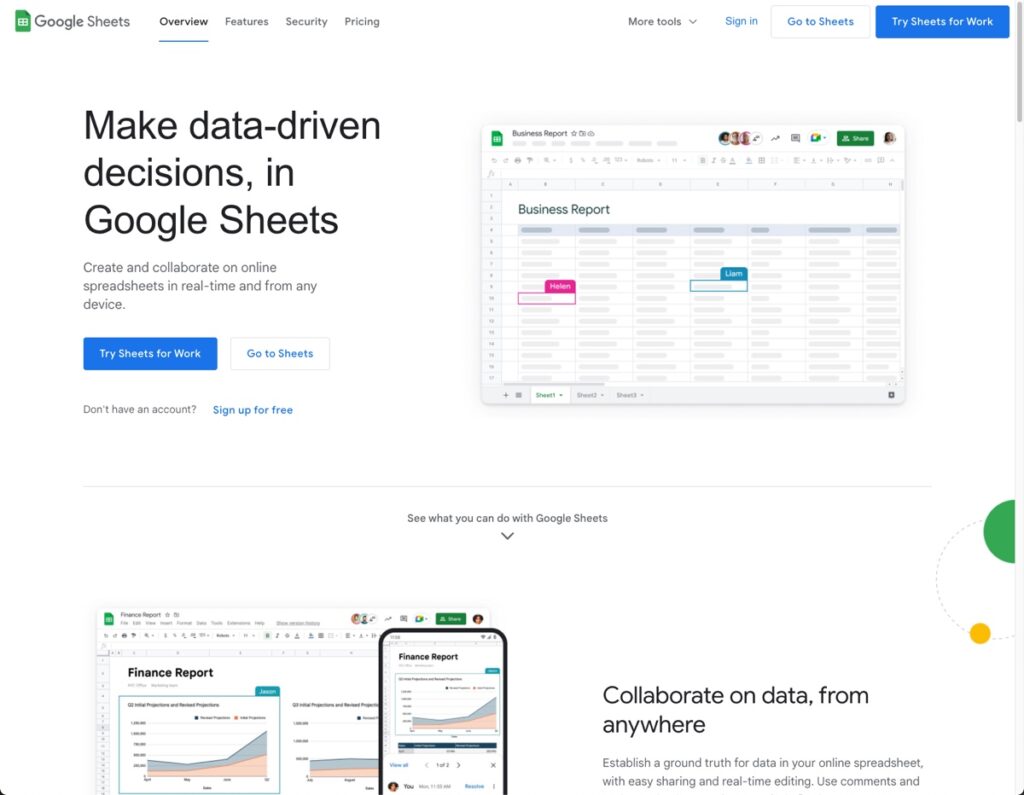
What is Google Sheets?
Google Sheets is a free, cloud-based spreadsheet application. That means you open it in your browser window like a regular webpage, but you have all the functionality of a full spreadsheet application for doing powerful data analysis. It really is the best of both worlds.
How is it different to Excel?
No doubt you’ve heard of Microsoft Excel, the long-established heavyweight of the spreadsheet world. It’s an incredibly powerful, versatile piece of software, used by approximately 750 million – 1 billion people worldwide. So yeah, a tough act to follow.
Google Sheets is similar in many ways, but also distinctly different in other areas. It has (mostly) the same set of functions and tools for working with data. In fact, some people mistakenly call it “Google Excel” or “Google spreadsheets.”
With the risk of getting into an opinionated debate about the strengths/weaknesses of each platform, here are a few key differences:
Google Sheets is cloud-based whereas Excel is a desktop program. With Sheets, you’ll no longer have versions of your work floating around. Everyone always sees the same, most up-to-date version of Sheets, showing the same spreadsheet data.
Collaboration is baked into Sheets, so it works extremely well. Excel is still trying to play catch up here.
Both have charting tools and Pivot Table tools for data analysis, although Excel’s are more powerful in both cases.
Excel can handle much bigger datasets than Sheets, which has a limit of 10 million cells.
Being a cloud-based program, Google Sheets integrates really well with other online Google services and third-party sites.
Both have scripting languages to extend their functionality and build custom tools. Google Sheets uses Apps Script (a variant of Javascript) and Excel uses VBA.
For the material we’ll cover in this article, there’s very little difference between the programs, however.
For a deep-dive into the differences between Excel and Google Sheets, have a look at ExcelToSheets.com
Why use Google Sheets?
How’s this for starters:
It’s free!
It’s collaborative, so teams can all see and work with the same spreadsheet in real-time.
It has enough features to do complex analysis, but…
…it’s also really easy to use.
Need more convincing? Here are 5 more reasons from Google themselves.
Can it still do advanced stuff?
Absolutely! You can build dashboards, write formulas that make your head spin and even build applications to automate your job. The sky’s the limit!
You’ll find lots of resources on this site for intermediate/advanced level users, as well as comprehensive online training courses.
Ok, where do I get it? How to create your first Google Sheet
Click on the Go To Google Sheets button in the middle of the screen. You’ll be prompted to login:
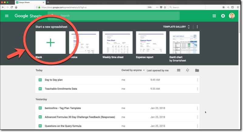
And then you arrive at the Google Sheets home screen, which will show any previous spreadsheets you’ve created.
Click the huge green plus button to create a new Google Sheet:
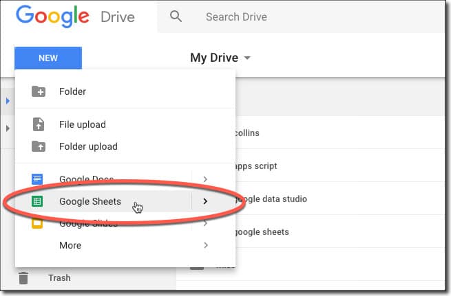
Opening your first Google Sheet from Drive
You can create new Google Sheets from your Drive folder by clicking on the blue NEW button:
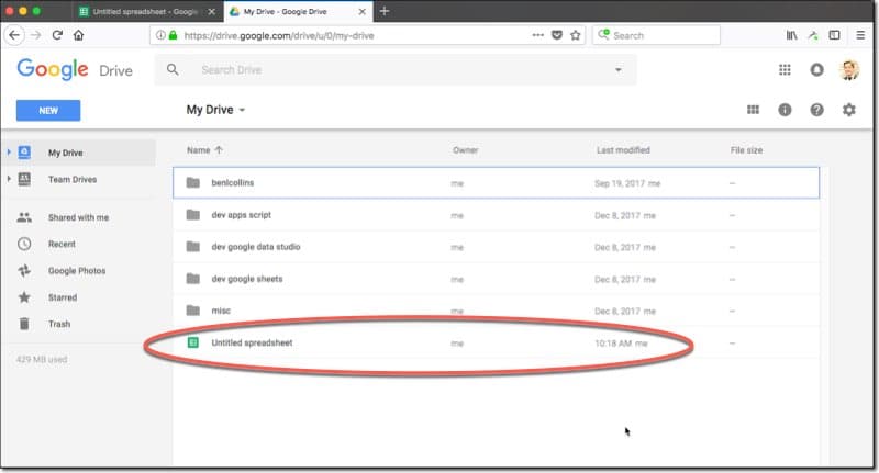
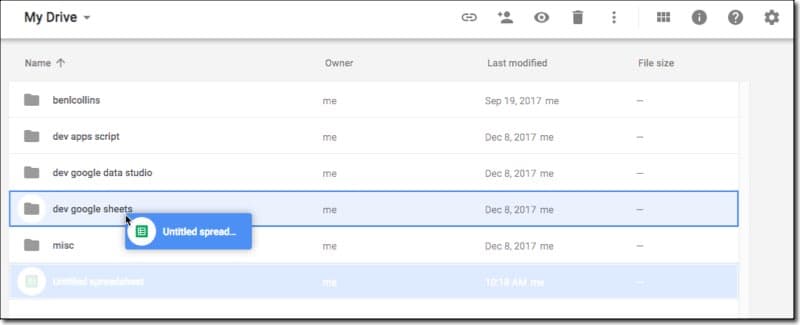
When you create a new Google Sheet, it’ll be created in your main Drive folder (your root folder):
(Note: Don’t panic if you don’t see the Sheet yet, it may not show up until you’ve renamed it. See next step on how to do this.)
Here you can drag it to a different folder if you wish (to keep things organized). Do this by clicking-and-holding the file, and dragging to where you want it to go:
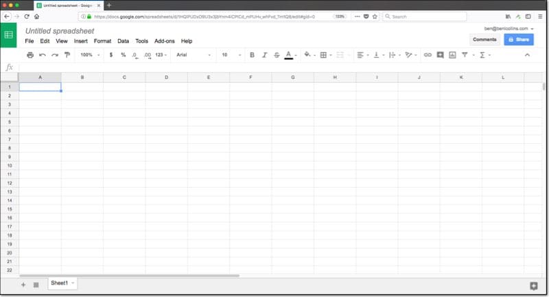
The Google Sheet editing window
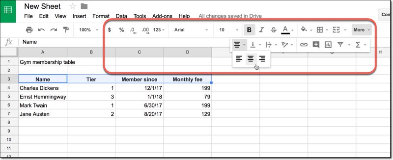
This is what your blank Google Sheet will look like:
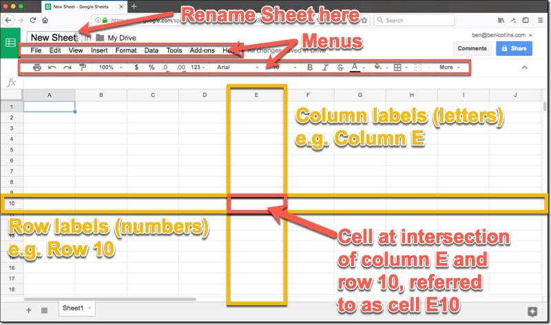
You can rename your Sheet in the top left corner. Click on where it says Untitled spreadsheet and type in whatever name you want to give your Sheet, in this example “New Sheet”.
So let’s introduce some key terminology and the fundamental concept upon which spreadsheets work:
There are two menu rows above your Sheet, of which we’ll see more further on in this tutorial.
The main window consists of a grid of cells. An individual cell is a single rectangle, at the intersection of one column and one row, and it’ll hold a single piece of data.
The columns are vertical ranges of cells, labeled by letters running across the top of the Sheet.
Rows are horizontal ranges of cells, labeled by numbers running down the left side of your Sheet.
In the example above, I highlighted column E and row 10.
** The fundamental concept of spreadsheets: **
Column E and row 10 intersect at one cell, and one cell only. Thus we can combine the column letter and row number to create a unique reference to this cell, E10. Now when we want to refer to this cell, for example to access data in this cell, we use the address E10 to do that.
Understand this and you understand spreadsheets. The rest is just details!
Entering, selecting, deleting and moving data
Now the fun really starts! Let’s start using this new blank sheet we’ve created.
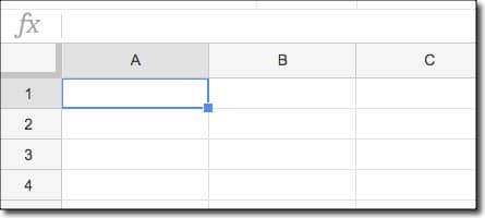
Click cell A1 (that’s the intersection of column A with row 1, the cell in the top left corner of the Sheet) and you’ll see a blue box around the cell, to indicate it’s highlighted:
Then you can simply start typing and you’ll see the data being entered into that cell:
Hit enter when you’ve finished entering data and you’ll move down to the next cell, having completed your data entry. If you hit the Tab key instead, you’ll move across one cell to the right!
It’s worth pointing out an important nuance here:
Clicking ONCE on the cell highlights the whole cell. Clicking TWICE enters into the cell, so you can select or work with the data only.
If you find yourself stuck inside a cell, you can press the ESCAPE key to deselect the contents and go up a level, to just having the cell selected.
Try it for yourself and see how the cursor shows up inside the cell when you double-click, allowing you to edit the data.
To delete the data we just entered, either click the cell once and hit the delete key, or, click the cell twice and then press the delete key until all your data is cleared out.
💡 Learn more Check out my brand new beginner’s course: Google Sheets Essentials. This is a 100% online, on-demand video training course designed specifically to help you boost your spreadsheet skills.
Help! I made a mistake
First of all, don’t panic!
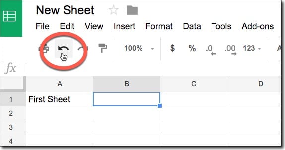
Google Sheets saves every step of your work so you can always go back a step (or two) if needed.
Press Cmd + Z if you’re on a Mac, or Ctrl + Z if you’re on a PC and you’ll undo your previous step. Keep pressing and you’ll simply go further back through your changes. (Pressing Cmd + Y on a Mac, or Ctrl + Y on a PC moves your forwards, to redo your last step.)
You can also undo using the Undo arrow on the menu:
Creating a basic table
Right, with all that in mind, it’s time for a quick exercise.
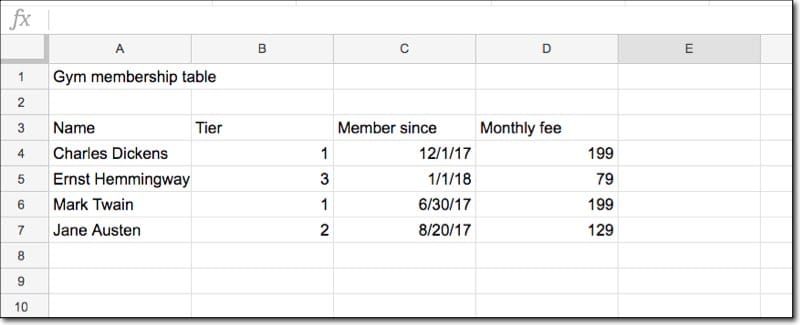
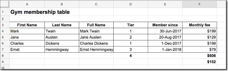
See if you can create the following table for our fictitious gym membership site, by entering the data into the correct cells (there is no formatting or other tricks used at this stage):
Feel free to use your own data if you wish. Also note that the dates entered above are in US format, with the Month first, so don’t worry if your table has the Day first.
2. How to use Google Sheets: The working environment
Changing the size, inserting, deleting, hiding/unhiding of columns and rows
To select a row or column, click on the number (rows) or letter (columns) of the row or column you want to select. This will highlight the whole row or column blue, to indicate you have it selected.
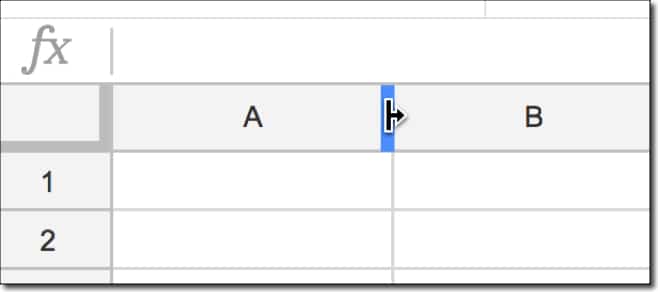
To change the width of a column, or height of a row, hover your cursor over the grey line denoting the edge of the column or row, until your cursor changes to look like this:
Then click and drag the cursor left or right to change the width of this column. It’s the same process to change the height of rows.
Pro-tip: To quickly change the column width to fit your cell contents, double-click when you’ve hovered over the grey line.
How to add columns in Google Sheets: To insert additional columns or rows, click on the existing column or row next to where you’d like to insert a new column or row. With the column or row selected (highlighted blue), right-click to bring up the options menu, then select Insert Before (or Insert After) for Columns, or Insert Above (or Insert Below) for Rows:
Adding extra rows and columns at end
If you reach the outer edges of a Google Sheet, you’ll notice the rows and/or columns stop. But don’t worry, you can add more.
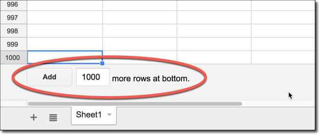
If you’ve scrolled all the way to the bottom of your Sheet (or added that much data), you’ll notice that you’re given 1,000 rows by default. There’s a button to add more rows if you need, either 1,000 as shown, or any number you wish (up to a limit, more on that below).
If you reach the right edge of the Sheet, i.e. the last column, then you add more columns in the standard way. Right-click a cell in the last column to bring up the menu and then choose to add a column to the right.
Pro-tip: If you want to add more than one column, there’s a trick to do it in one go. As an example, say you wanted to add three new columns to the right side of your Sheet, begin by highlighting the last three columns that are there already, then right-clicking and choosing to insert new columns. It’ll then insert three new columns for you!
Data Limit: Finally, keep in mind that each Google Sheet is limited to 10 million cells, which sounds like a lot but soon fills up. Anyway, you’ll find Sheets slows down considerably before reaching that limit. Most people report a slight slow down with tens of thousands of rows of data and complex formulas and models.
Adding/removing multiple sheets, renaming them
Super easy!
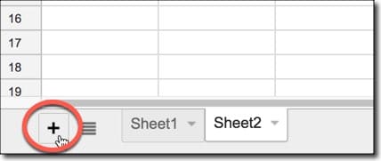
Click the big plus button in the bottom left of your Google Sheet to add a new Sheet (also called a Tab).
Why use multiple tabs within your Google Sheet?
Well, like a book with chapters on different topics, it can help separate different data and keep your Sheet organized.
For example, you might have a Sheet solely to record your global settings (any variables like name, email, tax rate, headcount…) and another for transactional data, and yet another for the analysis and charts.
The button with the three bars, next to the plus, is your index button, listing all of the tabs in your Google Sheet. This is super useful when you start having a lot of different tabs to manage.
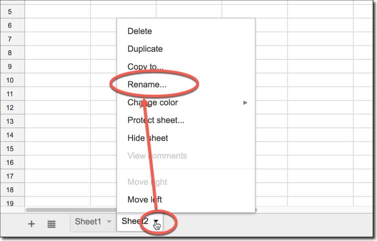
To rename a sheet, or delete a sheet, click the small arrow next to the name (e.g. Sheet1) to bring up the menu. Here you’ll see the option to rename, to delete, or even hide (and unhide) Sheets.
For naming, I try to indicate what’s in that tab, so use names like Settings, Dashboard, Charts, Raw Data.
Formatting
You’ll find all of the formatting options on the top toolbar, so you can center your headings, make them bold, format numbers as currency etc. You may find them all on one single row, or you may find some under the More button, as shown in this image:
They’re similar to a word processor and pretty self-explanatory. You can always hit undo if you make a mistake (Cmd + Z on Mac, or Ctrl + Z on PC).
Try the following to format our basic table:
> Make the heading bold and size 14px
> Center the column headings and make them bold
> Center the tier column
> Change the date format to 01-Jan-2018 (Hint: the date format is found under the button that says 123.)
> Add a dollar sign, $, to the fee column
> Add a border around the whole table.
Here’s a GIF to guide you:
(Note, you can also find the formatting options under the Format menu, between the Insert and Data menu options.)
Alternating colors
Let me show you the option to add alternating row colors (banding) to your tables.
Let’s apply it to our basic table, by highlighting the table and then from the menu:
Format > Alternating colors
as shown here:
Remember, a little bit of formatting goes a long way. If you Sheet is more readable and tidy, people will be more likely to understand it and absorb the information.
Removing formatting
This is my number 1 productivity tip in Google Sheets.
To remove all formatting from a cell (or range of cells), hit Cmd + \ on a Mac or Ctrl + \ on a PC.
This will save you so much time when you’re wanting to remove formatting that isn’t yours or that you no longer want or need.
3. How to use Google Sheets: Data and basic formulas
Different types of data
You’ve already seen different data types in Google Sheets in our basic table.
The key point to understand with spreadsheet data is that each cell contains the data itself, and a format applied to that data.
For example, suppose a cell contained:
2, or 2.00, or $2, or $2.00
In each case the underlying data is the number 2, but with a different format applied each time. If we add 2 to each of these cells we get back the number 4 in every case (with formatting applied).
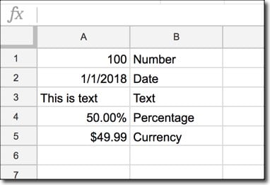
Basic data types in Google Sheets
You’ll notice that currency data, percentage data and even dates are actually just numbers under the hood (dates? Really? Yes, they are, but that’s a discussion for another day). They’re all right-aligned, hanging out on the right edge of their cell.
Text is left-aligned by default.
If you want to force something to be stored as text, you can prepend a single quote, ' before the cell contents. So typing in '0123 will show as 0123 in your cell and be left-aligned. If you omit the single quote mark, then it’ll be stored as a number and show up as 123 without the 0.
Doing math on numbers
Easy-peasy, just like you do on a calculator.
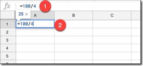
You click the cell you want to do your calculation in, type an equals sign (=) to indicate you’re performing a calculation and then type in your formula, e.g.
Notice how calculation will show in the formula bar (1) as well as in the cell (2).
You’ll notice that you get a preview of the answer (in this case, 25) above the formula.
Starting with functions: COUNT, SUM, AVERAGE
Technically you’ve already written your first formula in the section above on math calculations, but really, your formula career begins when you start using the built-in functions (of which there are hundreds!).
Returning to our basic table, let’s count how many members we have, what the total monthly fees are and what the average monthly fees are.
COUNT
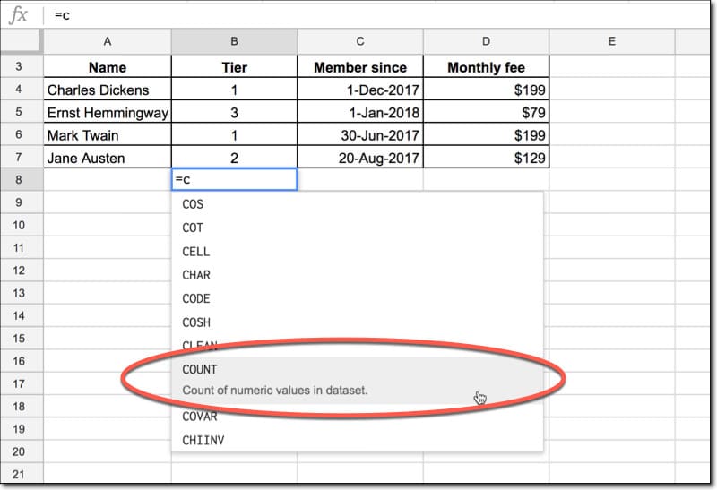
Click on cell B8, type an equals (=) and then start typing the word COUNT. You’ll notice an auto-complete menu comes up showing all of the functions beginning with C, like this:
You can either keep typing COUNT in full, or find it and select in from the list (hover over it and click on it OR hit enter OR hit tab).
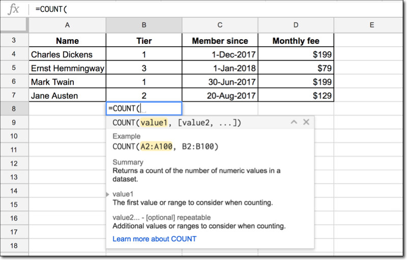
Next you’ll see the formula helper window show up, which tells you about the formula syntax and how to fill it in correctly:
In this case, the COUNT function is expecting a list of numeric values.
You have to select the range of cells you want to count. So click on B4, hold you mouse down and drag down to B7, so that the four cells are highlighted in orange and B4:B7 is showing up in your function:
Then, close the function with a closing bracket “)”:
=COUNT(B4:B7)
Note: COUNT is used to count numbers. If you want to count text (for example the names) then COUNT won’t work (it’ll give you a 0). Instead use COUNTA (with an A at the end), otherwise the method is the same.
SUM
Your turn! Try creating a total for the membership fees in cell D8. Follow the same process as the count function, except use SUM and highlight the values in column D.
=SUM(D4:D7)
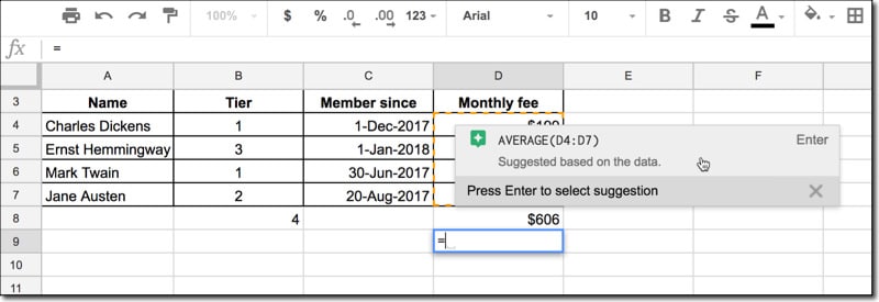
AVERAGE
You’re on a roll, so go ahead and calculate the average of the membership fees. Use the AVERAGE function in cell D9.
=AVERAGE(D4:D7)
Psst, you’ll notice that Google even helps you out sometimes and suggests the exact formula you were after:
Here you go:
If you make a mistake with your formula, you’ll see an errors message, probably something like #N/A, #REF!, #DIV/0 etc.
You’ll need to re-enter your formula and correct it before proceeding. These error messages do give a lot of context though, so they’re worth understanding.
What’s the difference between a function and a formula?
Well, both are used interchangeably and rather loosely so I wouldn’t get hung up on it.
For the pedantic, a function refers to the single method word (e.g. SUM) whereas a formula refers to the whole operation after the equals sign, often consisting of multiple functions.
Separating data with the Text to columns feature
Let’s suppose you wanted First Name and Last Name, rather than just simply Name as we have in our dead famous authors membership table. How do we go about doing that?
Well of course, as with everything in spreadsheets, there are lots of ways, but let me show you the easiest, using the Text to Columns feature.
Back to our basic table, create a new column to the right of Name before the Tier column, i.e. create a new, blank column B.
Highlight the four names and click:
Data > Split text to columns…
On the sub-menu that shows up choose SPACE and marvel at how Google Sheets separates the full name into a first and last name. Feel free to rename the columns First Name and Last Name too.
Combining cells
Oh, blast I hear you say! You meant to keep hold of that full Name column as well.
No problem, let’s learn how to combine text so we can rebuild it.
Insert a new blank column between B and C (between Last name and Tier) and call it Full Name, in cell C3.
Add this formula in cell C4:
= A4 & B4
That’s A4, Ampersand, B4.
What it does is combine the data in cell A4 with the data in cell B4 and output it in cell C4.
Hmm, but this gives an output like this:
CharlesDickens
That’s obviously not good enough! We need a space between the names!
Change the formula to this, by clicking right after the ampersand and adding double quote, space, double quote, ampersand:
= A4 & " " & B4
Here we’ve told Google Sheets to add a space into the mix, and the output now will be:
Charles Dickens
Voilà, that’s better!
Your formula is sitting pretty in cell C4, but how do you get it to work for the other rows?
Copy it!
You can either:
i) right-click, copy, move down to select the next cell, right click again, click paste, or
ii) Cmd + C (on Mac) or Ctrl + C (on PC), move down to select next cell, then Cmd + V (on Mac) or Ctrl + V (on PC), or
iii) drag the formula down by holding the little blue box at the bottom right corner of the blue highlighting around the original cell.
The neat thing is that as you copy this formula down, the cell references will change from row 4 to row 5, row 5 to row 6, etc., automatically! How cool is that!
(This is what’s known as relative references. More on that in section 5 below.)
Let’s see some of the unique, powerful features that Google Sheets has, as a cloud-based piece of software.
Comments (and Notes)
Want to add some context to numbers in the cells of your Sheets, without having to add extra columns or mess up your formatting?
Add a comment to a cell!
You can tag people (via their email address) who you want to see the comment too. They can reply and mark it resolved once it’s been acted upon.
You can also add simple notes to cells as well if you wish.
Comments and Notes can also be deleted when not required anymore.
To add a comment to a cell, first select the cell, then right click to bring up the menu of options. Select “Insert comment” and then simply type in your comment.
To tag somebody in your comment, type the plus sign (+) and their name or email address (you’ll see auto-complete options from your contacts, so you shouldn’t have to type in the whole email address).
You’ll notice a small orange triangle in the top right corner of the cell to indicate the comment. The comment will show up when you hover over this cell. If you click on the cell, it’ll also add orange shading to the cell background.
Comments can be edited, deleted, linked to, replied to and resolved (comment disappears from Sheet and is archived).
You can reach and control all the Comments in your Sheet from the big Comments button in the top right of the screen, next to the blue Share button.
(The first time you tag someone in a comment, you’ll be asked to share the Sheet with them. See more on this below.)
You can also add a note to cells in the same way (look for it in the menu next to Insert Comment). It’s like a pared down version of a comment, intended for your own reference.
Share your sheets
(If you just added a comment and tagged someone else, as shown above, then you may have already done this step!)
You can share your Google Sheets with other people. Since it’s on the cloud, they can access your Sheet and see the same, live Sheet that you’re in.
In other words if you make changes, they will show up automatically and in near real-time for everybody viewing the Sheet.
You can have multiple people viewing and working on the same Sheet.
Essentially you have three options to share you Sheet with:
View-only access, so that person can not change or comment on any data
Comment-only access, so that person can add comments but still not make any changes to the data in the Sheet
Editing access, so that person can make changes to the sheet (including comments)
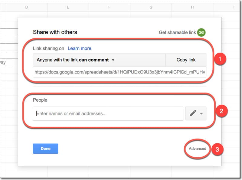
The Sharing options are found by clicking on the big blue button in the top right corner, which will open up the Sharing settings:
You can grab the link (the URL) to the Sheet, choose the share setting (view/comment/edit) and then share that link with people you want to see the Sheet. (1)
Or, you can enter someone’s email address directly, choose the share setting (view/comment/edit) and then share the Sheet directly with the person. (2)
If you want to review the sharing settings or have even more control, click the Advanced options buttons. (3)
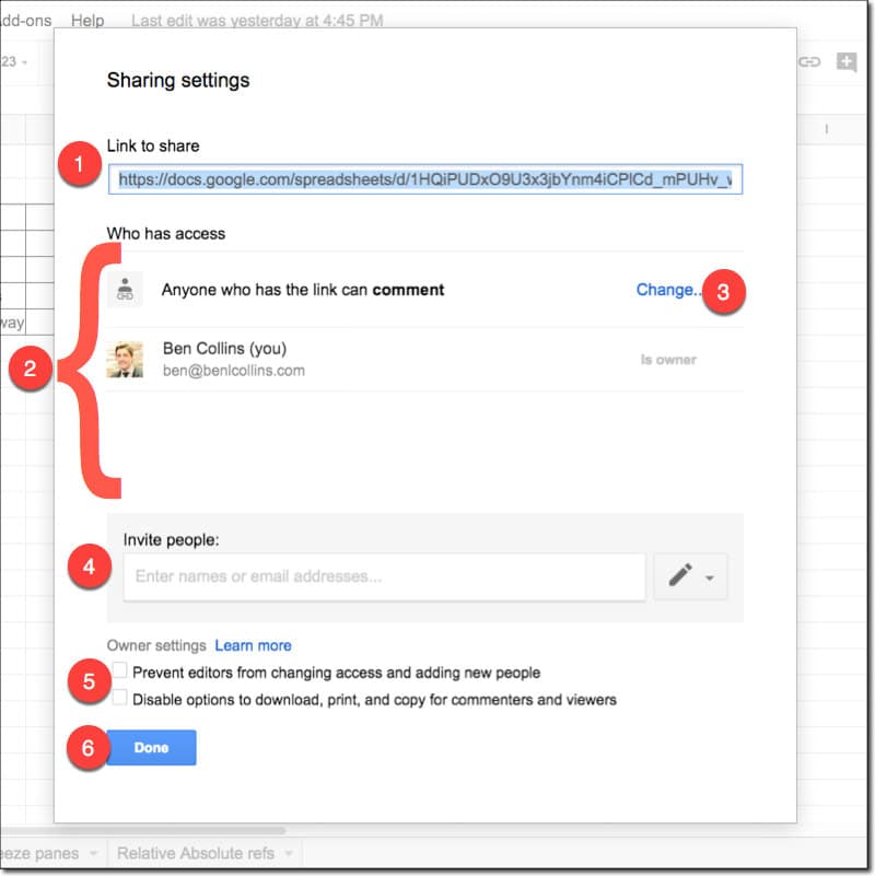
The Advanced sharing settings window:
Here you can:
> Grab the sharing link (1)
> Review who has access (2)
> Change the access rights of anyone listed (3)
> Invite new people to access the Sheet (4)
> Change the advanced owner settings, to restrict who can control the sharing settings and specific view/comment rights (5)
> Confirm when you’re finished (6)
I’ve used the link from the sharing settings to share the template for this tutorial with you!
Real-time Collaboration
Ok, so you’ve shared your Sheet with someone. If they open it whilst you’re still working in the Sheet you’ll see their cursor show up on whatever cell (or range) they’ve selected. It’ll be a different color, for example green to your blue.
If they enter data or delete data you’ll see it happening in real-time!
In this case my active cell is the blue-outlined cell. I see somebody else, denoted by the green-outlined cell, show up in this Sheet and enter data into a few cells before deleting it.
5. How to use Google Sheets: Intermediate techniques
Freeze panes
This is one of the most useful tricks you can learn in Google Sheets, which is why I’m recommending you learn it today.
Sooner or later you’ll work with a table of data that continues beyond the area you see on the screen (right now for example, I can see as far as row 26, but it depends on your screen size and other factors).
When you scroll down to look at data further down in your table, you lose the column headings off the top of your screen, and therefore can’t see the context of your columns.
Of course, scrolling up and down to see what the column headings are makes no sense. It’s a sure path to spreadsheet errors and insanity!
Have a look at this data table showing the tallest buildings in the world, which extends below the bottom of what you can see on a single screen in Sheets. Scrolling results in the heading row disappearing, so you no longer know which columns are which:
What you need to do is freeze the heading rows.
Thankfully it’s super easy.
Click on the row number of the row with your column headings in (e.g. row 3), then from the menu choose:
View > Freeze > Up to current row (3)
Now your headings will stay in place. Ah, that’s much better!
You can do the same with columns, if you wished to freeze names for example, so you can scroll horizontally across lots of columns of data.
Relative/Absolute references
This is arguably the hardest concept to grasp in this tutorial. If you understand it and can apply it, then you have a really good understanding of how spreadsheets work and you’re well on your way to being a skilled user.
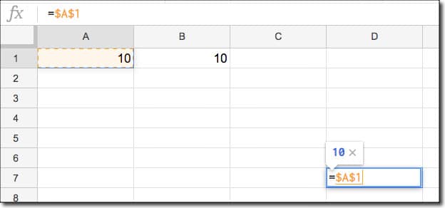
Suppose you have some data in cell A1 and you enter the following formula into cell B1:
= A1
This formula will retrieve whatever data is in cell A1 and show it in cell B1.
Now copy the formula (Cmd + C on a Mac, or Ctrl + C on a PC) and paste it (Cmd + V on a Mac, or Ctrl + V on a PC) somewhere else on your Sheet, for example cell D5.
Nothing will show up in D5. In fact you may be wondering whether your copy-paste worked. Have a look in the formula bar and you should now see this however:
= C5
The formula is there, but it points to a different cell, not A1, so does not show the data from A1.
But it still points to the cell that is ONE TO THE LEFT AND ON THE SAME ROW as the original formula.
Ah ha! Eureka!
The formula copied perfectly, keeping the same structure, pointing to the cell on the left.
This amazing property is called a relative reference, meaning it’s in relation to the cell where the formula is (e.g. one to the left).
That’s why you can drag formulas down columns and they’ll change automatically to calculate with data from their row.
Got that?
Now then, if you want to fix your formula (for example so it always point to cell A1) then you’ll want to use what’s called Absolute Referencing.
We lock the cell reference in the formula, so Google Sheets knows to not move the reference when the formula is moved.
The syntax uses a dollar sign, $, in front of the column reference and in front of the row reference to lock them each respectively, like so:
= $A$1
Now, wherever you copy this formula, the output will always point to cell A1 and return you the data from cell A1.
Note, you can just lock the column or just lock the row reference, and leave the other part as a relative reference, but that is beyond the scope of this tutorial.
Working with formulas across sheets
Sticking with the topic of referencing other cells for the moment, how does one go about linking to data on a different Sheet?
Returning once again to our basic gym membership table for dead famous authors, in Sheet 1, let’s retrieve the table heading and print it out in Sheet 2 with this formula, entered into cell A1 on Sheet 2:
= Sheet1!A1
Note the exclamation point at the end of the reference to Sheet1, i.e. Sheet1!
Now let’s do a simple sum of data on Sheet 1, but show our answer on Sheet 2.
In cell A3 in Sheet 2, enter the following formula:
= SUM( Sheet1!F4:F7 )
This will return the sum of the range of cells F4 to F7 in Sheet 1 and print out the answer in Sheet 2.
Basic conditional formatting
Conditional formatting is a powerful technique to apply different formats (for example background shading) to cells based on some conditions.
Let’s see an example of conditional formatting, that is, formatting based on variable conditions.
For example, in a financial model, you might show positive asset growth with a green font color and a light green background, whilst negative growth might be shown with red lettering on a light red background. This gives extra context to your numbers, and pre-attentive attributes (the colors) help to convey the message more efficiently.
Taking the plain copy of the membership table (hit Cmd + Z on a Mac, or Ctrl + Z on a PC to go back if you need), highlight the final column of the membership fee, then from the menu:
Format > Conditional formatting
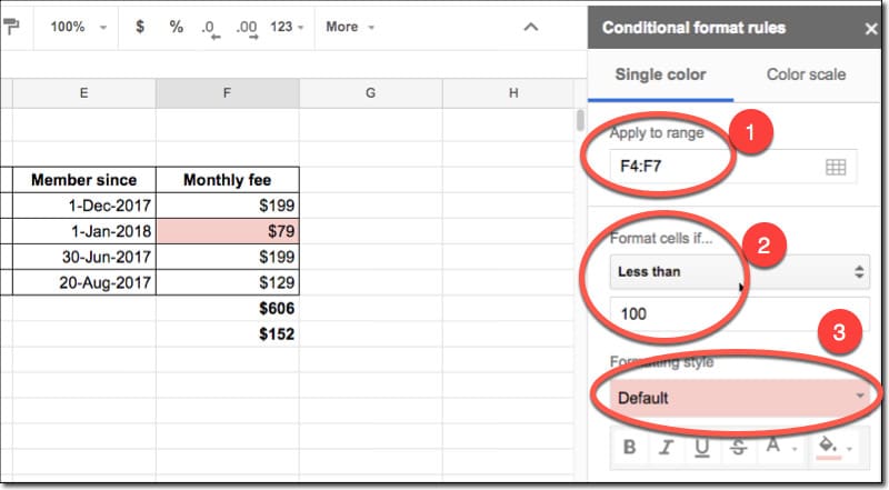
Here you can choose a rule, for example, values less than $100 and highlight them red:
Notice the range is shown (1), then a drop-down menu to choose a rule (2) and then the formatting option (3), which is default red in this case, although you can go completely custom if you choose.
The power of conditional formatting is to highlight data dynamically. The formatting is based on a rule, so if another value should drop below the threshold ($100 in this case), it will trigger the formatting rule and be highlighted red.
Sorting your data is a common request, for example to show transactions from highest revenue to lowest revenue, or customers with the greatest number to least number of purchases. Or to show suppliers in alphabetical order. You get the idea.
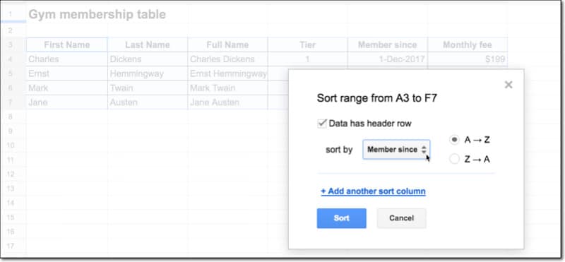
So let’s sort the dead famous authors gym membership table, from earliest members to most recent members, i.e. we’ll sort our table based on the date column.
Highlight the whole table, including the header row. Then from the menu:
Data > Sort range…
and be sure to check the “Data has header row” option. Then you can select the column you want to sort by, and sort option from A to Z, or Z to A.
This re-sorts the table, showing the earliest members first:
Filtering data
The next step after sorting your data is to filter it to hide the stuff you don’t want to see. Then you can just look at the data that is relevant to the problem at hand.
Taking the world’s tallest buildings data again, let’s apply a filter to only show skyscrapers built before the 2000s.
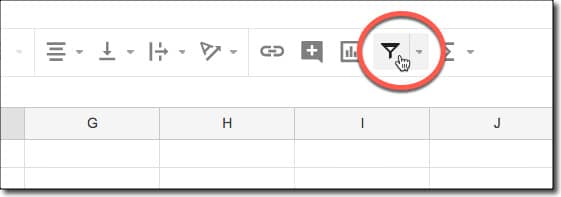
Click somewhere inside the data table (click on a cell containing data in the table), and then add the filters from the menu:
Data > Filter
or by clicking this icon on the menu bar above your Sheet:
You’ll notice a light green shading applied to row and column headings of your filtered table, and also a green border around your table. Most importantly though, you’ll now have little green filter buttons in each of your heading cells.
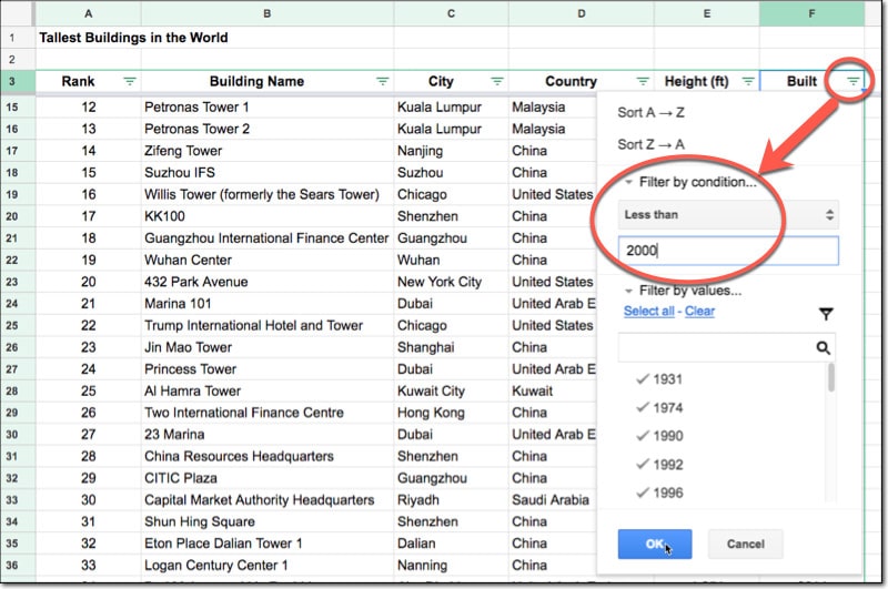
To filter out all the buildings built in the year 2000 or after, click the little green triangle next to the column heading Built, to bring up the filter menu.
You’ll notice you can manually select or de-select items to show. Let’s create a rule this time though.
Under the “Filter by condition” section, choose “Less than” and enter 2000 into the value box:
Hit OK.
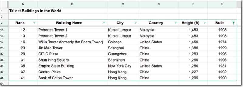
Ta-da!
You’ll see a reduced table with just 9 results. The 9 skyscrapers built before the year 2000:
To remove the filter, click the green triangle button again (now solid green) and under the “Filter by conditions” set the rule to “None”.
There’s also a native FILTER function, by which you can formulaically filter your data.
As a final exercise with the tallest building data, let’s draw a chart to show the buildings built by year, so we can see the trend graphically.
First, let’s sort the table by the year Built column, from oldest to newest. We can do this using the sort function that is provided in the menu when you click on the green triangle (from the filter).
Then highlight this single column called Built and from the menu:
Insert > Chart
This creates a default chart in your window and opens the chart editing tool in a sidebar.
Here you can change your data range and chart type, as well as a multitude of chart custom formatting options (which are also generally accessible by clicking on the elements directly in the chart).
A chart is an object in your Sheet now. Click it to select it, so it has a blue border around it. You can resize it and drag it to move it, just as you would with an image.
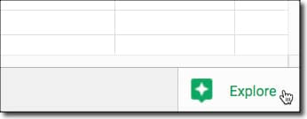
Using the Explore feature
The robots are coming!
Soon we won’t have to create complex formulas or charts ourselves. We’ll simply ask our Sheet to do it for us. Sound far-fetched?
Well, you can do that now! The future is here.
(Soon we won’t have to open Google Sheets at all, we’ll simply type, or more likely speak, our data questions into a dashboard console, and out will pop the answers, but I digress.)
Google Sheets has a feature called Explore, powered by Machine Learning/AI/Deep Learning/Neural Network sorcery, that will ingest your data, analyze it and show you some common answers (like the SUM, COUNTs etc. we’ve seen so far) and basic charts:
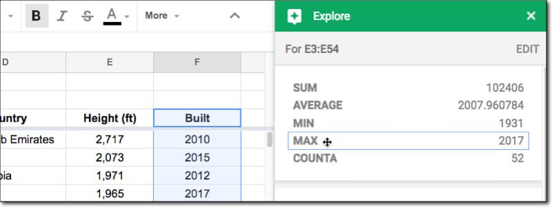
Let’s see an example, using the data about the world’s tallest buildings. Highlighting the column showing the years when each skyscraper was built and then clicking on the Explore button (bottom right corner) leads to these insights:
52 buildings in my set. The earliest tower on the list was built in 1931 (the venerable Empire State Building!) and the most recent was built in 2017. The average of all the years built is 2007.
Some interesting and useful data points, without having to do a lick of work!
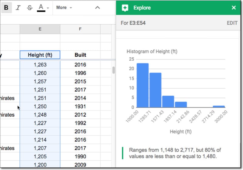
I mentioned charts, so let’s see an example of that with the Height (ft) column. Google Sheets Explore creates a Histogram for us, showing the distribution of tower heights:
We also get this interesting and insightful summary:
“Ranges from 1,148 to 2,717, but 80% of values are less than or equal to 1,480.”
Wow! At a glance, we have the min and max heights, but more impressive, we know that 80% are under 1,480ft tall.
Not all of the “insights” are useful, and I don’t use this feature much myself yet, but it shows a glimpse of how we’ll all work with Sheets in the future.
If you’re still not worried about AI taking over your job (whether that’s data analysis work or something else) in the next 10 to 50 years, then have a read of this article.
BONUS: VLOOKUP
No “How to use Google Sheets” article would be complete without at least a quick look at the VLOOKUP function.
Why?
Because it’s the most famous function. Tell anyone you work with data and spreadsheets and they’ll immediately ask, “yes, but do you know how to do a VLOOKUP?”
It’s a good bellwether for spreadsheet competency, even though there are ultimately better ways to work with data. It’s also a relatively advanced formula compared to what we’ve seen so far, so if you can understand it, it bodes well.
What does it do then?
It’s used to search for a term and return information about that term from a different table.
Generally, it’s used when you have two tables that share some common attribute (e.g. a name, ID number, or email), but otherwise, store different information. Suppose you want to bring this information together though. Well, you can, and you link the information via that common attribute.
One table might have details an employee’s name and address, and the other table might have their name and work details like title and salary. You can use the VLOOKUP function to bring these bits of data together in a single table.
In words: you select a search term that you search for in the first column of the search table. If you find it, you return a piece of information from the search table that relates to the search term (because it’s on the same row). The column number refers to which column of the search table you return the data from (1 being the column you searched in, so typically this number is 2 or greater).
Let’s see an example, by adding addresses to the dead famous authors’ gym membership table.
I’ve added a second table to Sheet 1, showing the addresses of our dead famous authors. What I’d like to do is add that data to the original gym table.
I want to do it efficiently with the VLOOKUP formula, rather than adding them manually. Not only is it much, much faster with larger tables (imagine ten thousand rows of data), but it’s also less error-prone.
The address table is in columns I and J, with the names in column I and addresses in column J.
So I’ll search for my author name in column I and return the address from column J, and print the output into whichever cell I created my formula in.
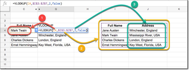
The formula is:
= VLOOKUP( C4, $I$3:$J$7, 2, FALSE )
And this is what’s happening:
I search for the name (1) in the search table (2) and return the data from column 2 of the search table (3).
I don’t expect you to understand all of this immediately (and there’s a lot more to this formula than what I’ve shown here), but if you try it out and persevere, you’ll get there and realize it’s actually not too difficult.
(The FALSE argument, the final piece of information in the VLOOKUP formula means you want to do an exact match. 99.9% of the time you use a VLOOKUP, you’ll want to use FALSE.)
💡 Learn more Check out my brand new beginner’s course: Google Sheets Essentials. This is a 100% online, on-demand video training course designed specifically to help you boost your spreadsheet skills.
The old adage “Practice makes perfect” is as true for Google Sheets as anything else, so hop to it!
Keep up-to-date with new articles, course launches and exclusive offers, by signing up for my Google Sheets newsletter, and get my free Google Sheets ebook with 100 tips.
In this API tutorial for beginners, you’ll learn how to connect to APIs using Google Apps Script, to retrieve data from a third-party and display it in your Google Sheet.
Example 1 shows you how to use Google Apps Script to connect to a simple API to retrieve some data and show it in Google Sheets:
In Example 2, we’ll use Google Apps Script to build a music discovery application using the iTunes API:
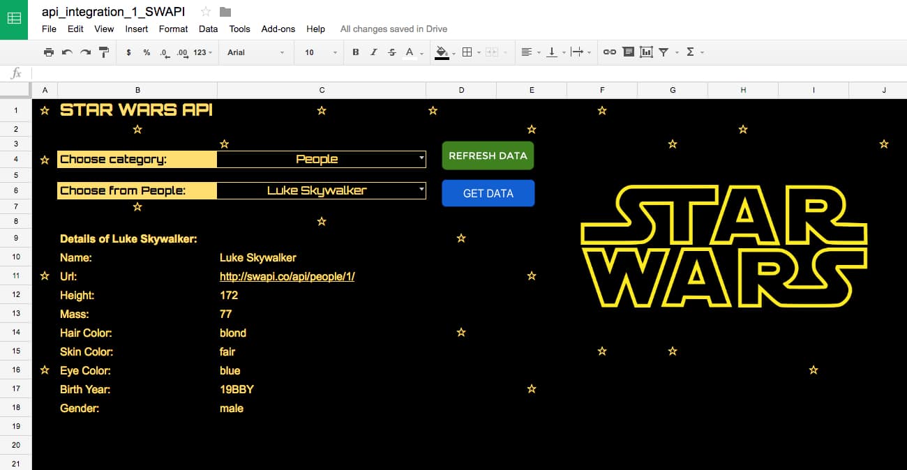
Finally, in example 3, I’ll leave you to have a go at building a Star Wars data explorer application, with a few hints:
API tutorial for beginners: what is an API?
You’ve probably heard the term API before. Maybe you’ve heard how tech companies use them when they pipe data between their applications. Or how companies build complex systems from many smaller micro-services linked by APIs, rather than as single, monolithic programs nowadays.
API stands for “Application Program Interface”, and the term commonly refers to web URLs that can be used to access raw data. Basically, the API is an interface that provides raw data for the public to use (although many require some form of API authentication).
As third-party software developers, we can access an organization’s API and use their data within our own applications.
The good news is that there are plenty of simple APIs out there, which we can cut our teeth on. We’ll see three of them in this beginner api tutorial.
We can connect a Google Sheet to an API and bring data back from that API (e.g. iTunes) into our Google Sheet using Google Apps Script. It’s fun and really satisfying if you’re new to this world.
Does coding fill you with dread? In that case, you can still achieve your goals using a no-code option to sync live data into Google Sheets. Check out Coefficient’s sidebar extension that offers Google Sheets connectors for CRMs, BI tools, databases, payment platforms, and more.
Example 1: Connecting Google Sheets to the Numbers API
We’re going to start with something super simple in this beginner api tutorial, so you can focus on the data and not get lost in lines and lines of code.
Let’s write a short program that calls the Numbers API and requests a basic math fact.
Step 1: Open a new Sheet
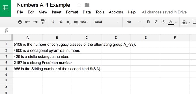
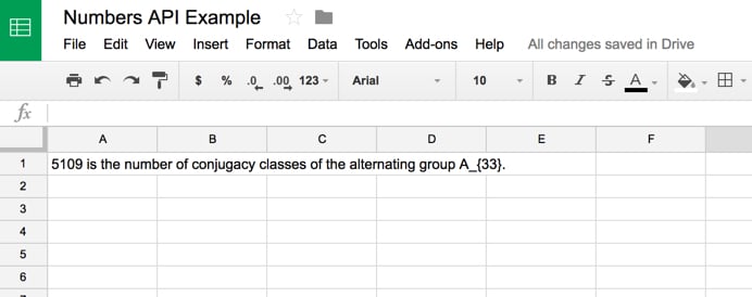
Open a new blank Google Sheet and rename it: Numbers API Example
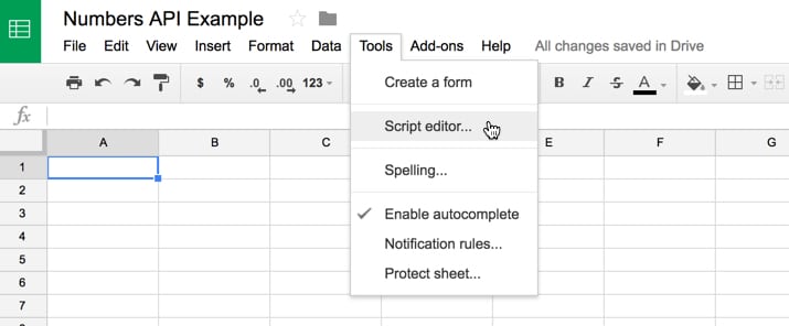
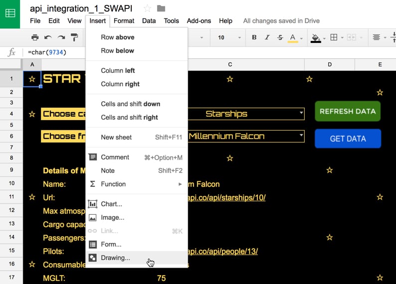
Step 2: Go to the Apps Script editor
Navigate to Tools > Script Editor...
Step 3: Name your project
A new tab opens and this is where we’ll write our code. Name the project: Numbers API Example
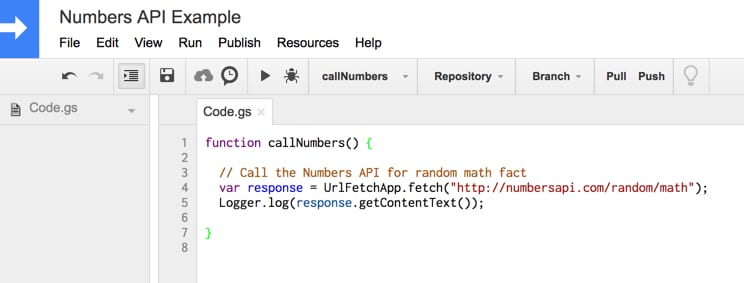
Step 4: Add API example code
Remove all the code that is currently in the Code.gs file, and replace it with this:
function callNumbers() {

  // Call the Numbers API for random math fact
  var response = UrlFetchApp.fetch("http://numbersapi.com/random/math");
  Logger.log(response.getContentText());

}
We’re using the UrlFetchApp class to communicate with other applications on the internet to access resources, to fetch a URL.
Now your code window should look like this:
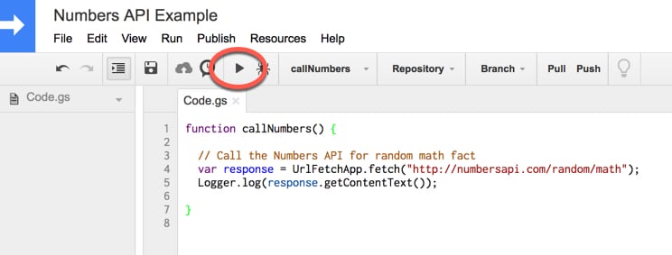
Step 5: Run your function
Run the function by clicking the play button in the toolbar:
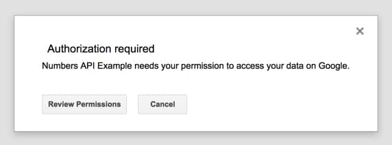
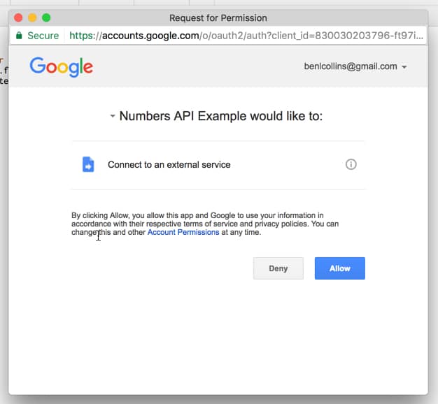
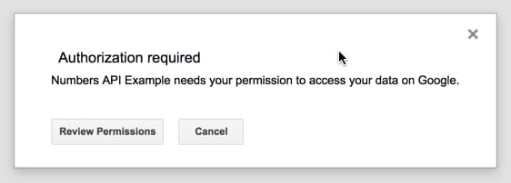
Step 6: Authorize your script
This will prompt you to authorize your script to connect to an external service. Click “Review Permissions” and then “Allow” to continue.
Step 7: View the logs
Congratulations, your program has now run. It’s sent a request to a third party for some data (in this case a random math fact) and that service has responded with that data.
But wait, where is it? How do we see that data?
Well, you’ll notice line 5 of our code above was Logger.log(....) which means that we’ve recorded the response text in our log files.
So let’s check it out.
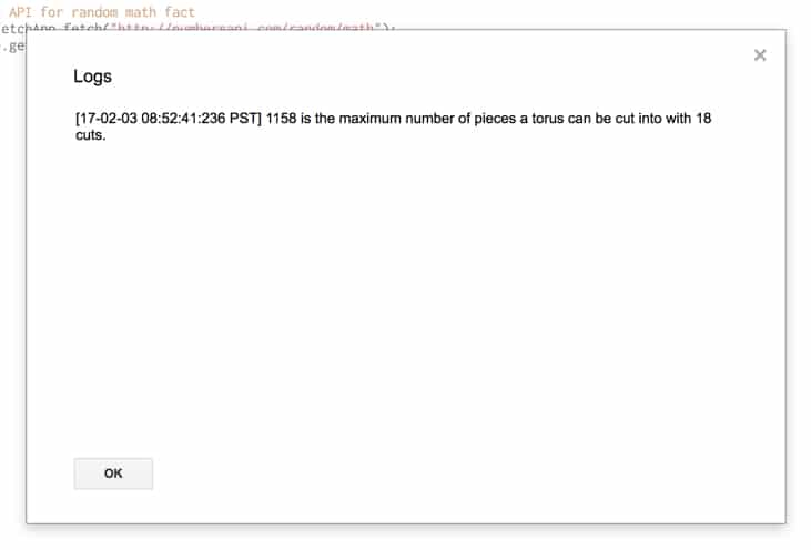
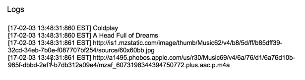
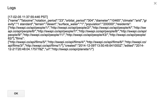
Go to menu button Execution Log
You’ll see your answer (you may of course have a different fact):
[17-02-03 08:52:41:236 PST] 1158 is the maximum number of pieces a torus can be cut into with 18 cuts.
which looks like this in the popup window:
Great! Try running it a few times, check the logs and you’ll see different facts.
Next, try changing the URL to these examples to see some different data in the response:
You can also drop these directly into your browser if you want to play around with them. More info at the Numbers API page.
So, what if we want to print the result to our spreadsheet?
Well, that’s pretty easy.
Step 8: Add data to Sheet
Add these few lines of code (lines 7, 8 and 9) underneath your existing code:
function callNumbers() {

  // Call the Numbers API for random math fact
  var response = UrlFetchApp.fetch("http://numbersapi.com/random/math");
  Logger.log(response.getContentText());

  var fact = response.getContentText();
  var sheet = SpreadsheetApp.getActiveSheet();
  sheet.getRange(1,1).setValue([fact]);

}
Line 7 simply assigns the response text (our data) to a variable called fact, so we can refer to it using that name.
Line 8 gets hold of our current active sheet (Sheet1 of Numbers API Example spreadsheet) and assigns it to a variable called sheet, so that we can access it using that name.
Finally in line 9, we get cell A1 (range at 1,1) and set the value in that cell to equal the variable fact, which holds the response text.
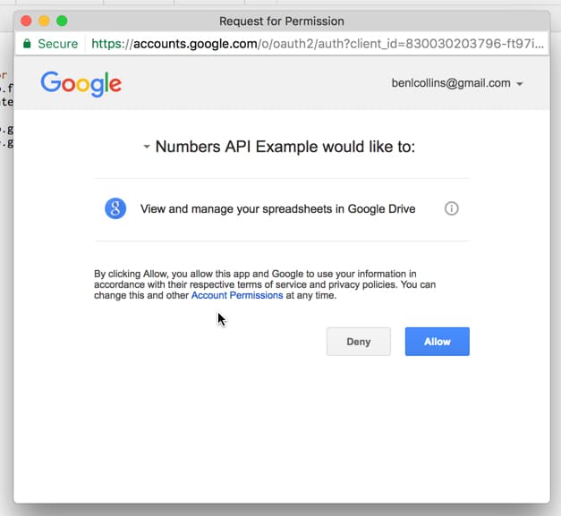
Step 9: Run & re-authorize
Run your program again. You’ll be prompted to allow your script to view and manage your spreadsheets in Google Drive, so click Allow:
Step 10: See external data in your Sheet
You should now get the random fact showing up in your Google Sheet:
How cool is that!
To recap our progress so far in this API Tutorial for Beginners: We’ve requested data from a third-party service on the internet. That service has replied with the data we wanted and now we’ve output that into our Google Sheet!
Step 11: Copy data into new cell
The script as it’s written in this API Tutorial for Beginners will always overwrite cell A1 with your new fact every time you run the program. If you want to create a list and keep adding new facts under existing ones, then make this minor change to line 9 of your code (shown below), to write the answer into the first blank row:
function callNumbers() {

  // Call the Numbers API for random math fact
  var response = UrlFetchApp.fetch("http://numbersapi.com/random/math");
  Logger.log(response.getContentText());

  var fact = response.getContentText();
  var sheet = SpreadsheetApp.getActiveSheet();
  sheet.getRange(sheet.getLastRow() + 1,1).setValue([fact]);

}
Your output now will look like this:
One last thing we might want to do with this application is add a menu to our Google Sheet, so we can run the script from there rather than the script editor window. It’s nice and easy!
Step 12: Add the code for a custom menu
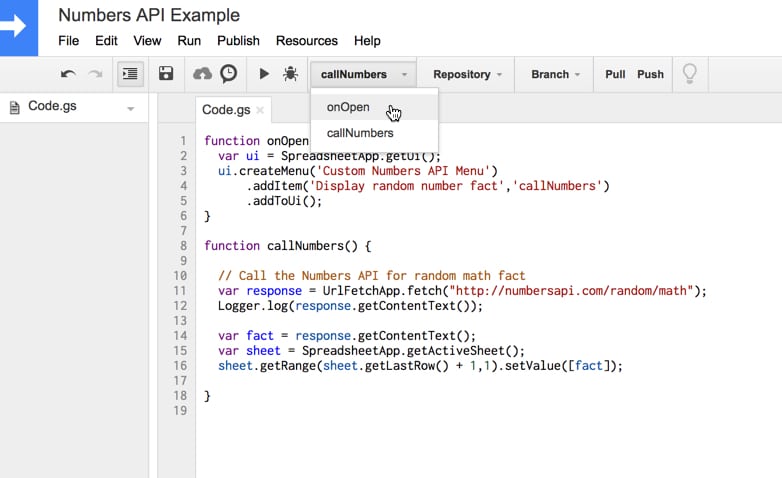
Add the following code in your script editor:
function onOpen() {
  var ui = SpreadsheetApp.getUi();
  ui.createMenu('Custom Numbers API Menu')
      .addItem('Display random number fact','callNumbers')
      .addToUi();
}
Your final code for the Numbers API script should now match this code on GitHub.
Step 13: Add the custom menu
Run the onOpen function, which will add the menu to the spreadsheet. We only need to do this step once.
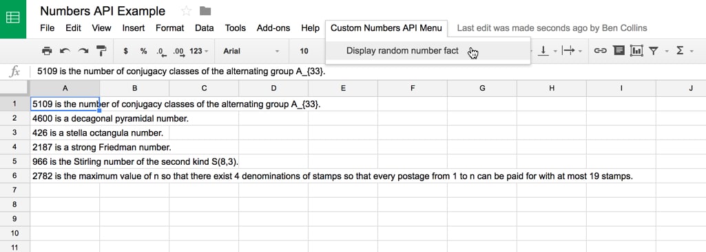
Step 14: Run your script from the custom menu
Use the new menu to run your script from the Google Sheet and watch random facts pop-up in your Google Sheet!
Alright, ready to try something a little harder?
Let’s build ourselves a music discovery application in Google Sheets.
Example 2: Music Discovery Application using the iTunes API
This application retrieves the name of an artist from the Google Sheet, sends a request to the iTunes API to retrieve information about that artist and return it. It then displays the albums, song titles, artwork and even adds a link to sample that track:
It’s actually not as difficult as it looks.
Getting started with the iTunes API Explorer
Start with a blank Google Sheet, name it “iTunes API Explorer” and open up the Google Apps Script editor.
Clear out the existing Google Apps Script code and paste in this code to start with:
function calliTunes() {

  // Call the iTunes API
  var response = UrlFetchApp.fetch("https://itunes.apple.com/search?term=coldplay");
  Logger.log(response.getContentText());
}
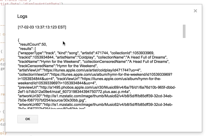
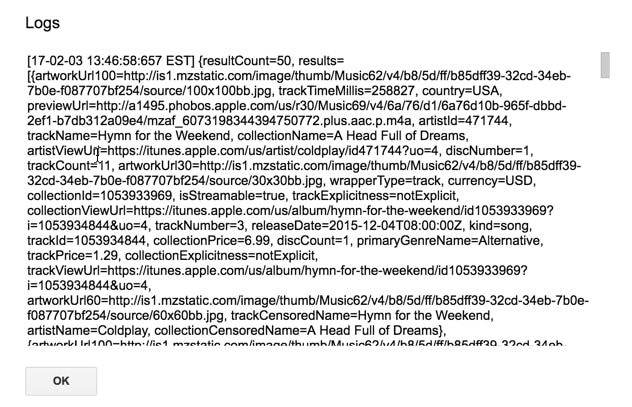
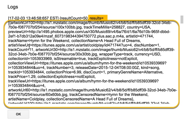
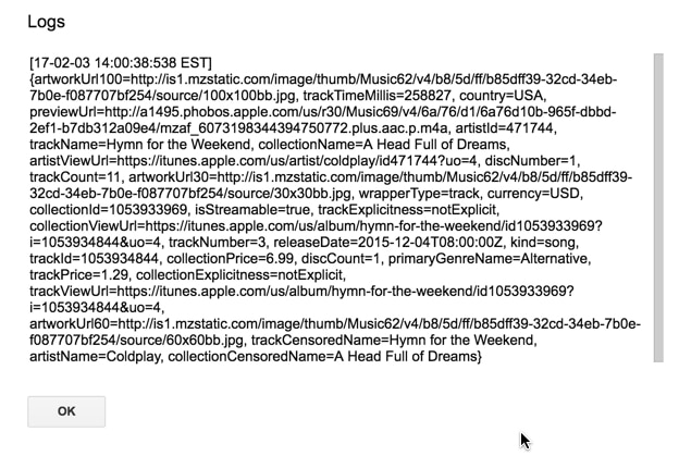
Run the program and accept the required permissions. You’ll get an output like this:
Woah, there’s a lot more data being returned this time so we’re going to need to sift through it to extract the bits we want.
Parsing the iTunes data
So try this. Update your code to parse the data and pull out certain bits of information:
function calliTunes() {

  // Call the iTunes API
  var response = UrlFetchApp.fetch("https://itunes.apple.com/search?term=coldplay");

  // Parse the JSON reply
  var json = response.getContentText();
  var data = JSON.parse(json);

  Logger.log(data);
  Logger.log(data["results"]);
  Logger.log(data["results"][0]);
  Logger.log(data["results"][0]["artistName"]);
  Logger.log(data["results"][0]["collectionName"]);
  Logger.log(data["results"][0]["artworkUrl60"]);
  Logger.log(data["results"][0]["previewUrl"]);

}
Line 4: We send a request to the iTunes API to search for Coldplay data. The API responds with that data and we assign it to a variable called response, so we can use that name to refer to it.
Lines 7 and 8: We get the context text out of the response data and then parse the JSON string response to get the native object representation. This allows us to extract out different bits of the data.
So, looking first at the data object (line 10):
You can see it’s an object with the curly brace at the start {
This will make it easier to see the details you’re extracting.
Putting this altogether in an application
If we want to build the application that’s showing in the GIF at the top of this post, then there are a few steps we need to go through:
Setup the Google Sheet
Retrieve the artist name from the Google Sheet with Google Apps Script
Request data from iTunes for this artist with Google Apps Script
Parse the response to extract the relevant data object with Google Apps Script
Extract the specific details we want (album name, song title, album artwork, preview url)
Clear out any previous results in the Google Sheet before showing the new results
Display the new results in our Google Sheet
Add a custom menu to run the program from the Google Sheet, not the script editor
It’s always a good idea to write out a plan like this before you commit to writing any lines of code.
That way you can think through the whole application and what it’s going to do, which allows you to make efficient choices with how you setup your code.
So the first thing to do is setup a Google Sheet. I’ll leave this up to you, but here’s a screenshot of my basic Google Sheet setup:
The important thing to note is the location of the cell where a user types in the artist name (11th row, 2nd column) as we’ll be referring to that in our code.
iTunes API Explorer code
And here’s the Google Apps Script code for our application:
// --------------------------------------------------------------------------------------------------
//
// iTunes Music Discovery Application in Google Sheets
//
// --------------------------------------------------------------------------------------------------

// custom menu
function onOpen() {
  var ui = SpreadsheetApp.getUi();
  ui.createMenu('Custom iTunes Menu')
      .addItem('Get Artist Data','displayArtistData')
      .addToUi();
}

// function to call iTunes API
function calliTunesAPI(artist) {

  // Call the iTunes API
  var response = UrlFetchApp.fetch("https://itunes.apple.com/search?term=" + artist + "&limit=200");

  // Parse the JSON reply
  var json = response.getContentText();
  return JSON.parse(json);

}


function displayArtistData() {

  // pick up the search term from the Google Sheet
  var ss = SpreadsheetApp.getActiveSpreadsheet();
  var sheet = ss.getActiveSheet();

  var artist = sheet.getRange(11,2).getValue();

  var tracks = calliTunesAPI(artist);

  var results = tracks["results"];

  var output = []

  results.forEach(function(elem,i) {
    var image = '=image("' + elem["artworkUrl60"] + '",4,60,60)';
    var hyperlink = '=hyperlink("' + elem["previewUrl"] + '","Listen to preview")';
    output.push([elem["artistName"],elem["collectionName"],elem["trackName"],image,hyperlink]);
    sheet.setRowHeight(i+15,65);
  });

  // sort by album
  var sortedOutput = output.sort( function(a,b) {

    var albumA = (a[1]) ? a[1] : 'Not known';  // in case album name undefined
    var albumB = (b[1]) ? b[1] : 'Not known';  // in case album name undefined

    if (albumA < albumB) { return -1; } else if (albumA > albumB) {
      return 1;
    }
    // names are equal
    return 0;
  });

  // adds an index number to the array
  sortedOutput.forEach(function(elem,i) {
    elem.unshift(i + 1);
  });

  var len = sortedOutput.length;

  // clear any previous content
  sheet.getRange(15,1,500,6).clearContent();

  // paste in the values
  sheet.getRange(15,1,len,6).setValues(sortedOutput);

  // formatting
  sheet.getRange(15,1,500,6).setVerticalAlignment("middle");
  sheet.getRange(15,5,500,1).setHorizontalAlignment("center");
  sheet.getRange(15,2,len,3).setWrap(true);

}
Let’s talk about a few of the key lines of code in this program:
Lines 16 – 25 describe a function that takes an artist name, calls the API with this artist name and then returns the search results from the API. I’ve encapsulated this as a separate function so I can potentially re-use it elsewhere in my program.
The main program starts on line 28.
On line 34, I retrieve the name of the artist that has been entered on the Google Sheet, and we call our API function with this name on line 36.
On lines 42 – 47, I take the results returned by the API, loop over them and pull out just the details I want (artist name, album name, song title, album artwork and preview track). I push all of this into a new array called output.
Next I sort and add an index to the array, although both of these are not mandatory steps.
On line 68, I clear out any previous content in my sheet.
Then on line 71, I paste in the new data, starting at row 15.
Finally, lines 74 – 76 format the newly pasted data, so that the images have space to show properly.
Run the onOpen() function from the script editor once to add the custom menu to your Google Sheet. Then you’ll be able to run your iTunes code from the Google Sheet:
Now you can run the program to search for your favorite artist!
Example 3: Star Wars data explorer using the Star Wars API
This one is a lot of fun! Definitely the most fun example in this API Tutorial for Beginners.
The Star Wars API is a database of all the films, people, planets, starships, species and vehicles in the Star Wars films. It’s super easy to query and the returned data is very friendly.
It’s a little easier than the iTunes API because the data returned is smaller and more manageable, and therefore easier to parse when you first get hold of it.
Getting started with the Star Wars API
As with both the previous APIs, start with a simple call to see what the API returns:
/*
 * Step 1:
 * Most basic call to the API
 */
function swapi() {

  // Call the Star Wars API
  var response = UrlFetchApp.fetch("http://swapi.dev/api/planets/1/");
  Logger.log(response.getContentText());
}
The data returned looks like this:
So, it’s relatively easy to get the different pieces of data you want, with code like this:
/*
 * Step 2:
 * Same basic call to the API
 * Parse the JSON reply
 */
function swapi() {

  // Call the Star Wars API
  var response = UrlFetchApp.fetch("http://swapi.dev/api/planets/1/");

  // Parse the JSON reply
  var json = response.getContentText();
  var data = JSON.parse(json);
  Logger.log(data);
  Logger.log(data.name);
  Logger.log(data.population);
  Logger.log(data.terrain);
}
Well, that should be enough of a hint for you to give this one a go!
Some other tips
In addition to custom menus to run scripts from your Google Sheet, you can add Google Sheets buttons and connect them to a script to run the script when they are clicked. That’s what I’ve done in this example.
On the menu, Insert > Drawing...
Create a button using the rectangle tool:
Finally, right click the drawing when it’s showing in your sheet, and choose Assign Script and type in the name of the function you want to run:
What else?
Use this CHAR formula to add stars to your Google Sheet:
=CHAR(9734)
I used the font “Orbitron” across the whole worksheet and, whilst it’s not a Star Wars font, it still has that space-feel to it.
The big Star Wars logo is simply created by merging a bunch of cells and using the IMAGE() formula with a suitable image from the web.
Let me know in the comments what you do with all these different APIs!
Disclosure: Some of the links in this post are affiliate links, meaning I’ll get a small commission if you click the link and subsequently signup to use that vendor’s service. I only do this for tools I use myself and wholeheartedly recommend.
The Google Sheets Filter function is a powerful function we can use to filter our data. The Google Sheets Filter function will take your dataset and return (i.e. show you) only the rows of data that meet the criteria you specify (e.g. just rows corresponding to Customer A).
Suppose we want to retrieve all values above a certain threshold? Or values that were greater than average? Or all even, or odd, values?
The Google Sheets Filter function can easily do all of these, and more, with a single formula.
In this example, we have a range of values in column A and we want to extract specific values from that range, for example the numbers that are greater than average, or only the even numbers.
The filter formula will return only the values that satisfy the conditions we set. It takes two arguments, firstly the full range of values we want to filter and secondly the conditions we’re going to apply. The syntax is:
=FILTER("range of values", "condition 1", ["condition 2", ...])
where Condition 2 onwards are all optional i.e. the Filter function only requires 1 condition to test but can accept more.
How do I use the Filter function in Google Sheets?
For example in the image above, here are the conditions and corresponding formulas:
Can I test multiple conditions inside a Google Sheets FILTER function?
Absolutely!
For example, using the basic data above, we could display all the 200-values (i.e. values between 200 and 300) with this formula:
=FILTER(A3:A21, A3:A21>200, A3:A21<300)
Can I test multiple columns in a Filter function?
Yes, simply add them as additional criteria to test. For example in the following image there are two columns of exam scores. The Filter function used returns all the rows where the score is over 50 in both columns:
The formula is:
=FILTER(A1:B20,A1:A20 > 50,B1:B20 > 50)
Note, using the Filter function with multiple columns like this demonstrates how to use AND logic with the Filter function. Show me all the data where criteria 1 AND criteria 2 (AND criteria 3...) are true.
Can I reference a criteria cell with the Filter function in Google Sheets?
Instead of hard-coding a value in the criteria, you can simply reference another cell which contains the test criteria. That way you can easily change the test criteria or use other parts of your spreadsheet analysis to drive the Filter function.
For example, in this image the Filter function looks to cell E1 for the test criteria, in this case 70, and returns all the values that exceed that score, i.e. everything over 70.
The formula in this example is:
=FILTER(A1:A20,A1:A20 > E1)
Can I do a filter of a filter?
Yes, you can!
Use the output of your first filter as the range argument of your second filter, like this:
Advanced Filter Examples in Google Sheets
How to use an advanced filter with an OR condition in Google Sheets. Knowing the trick will save you hours, so you can filter multiple conditions easily.
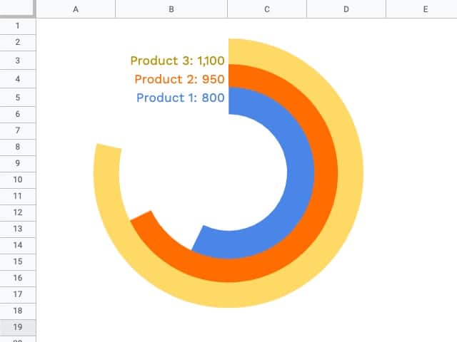
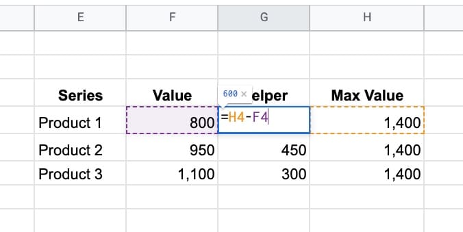
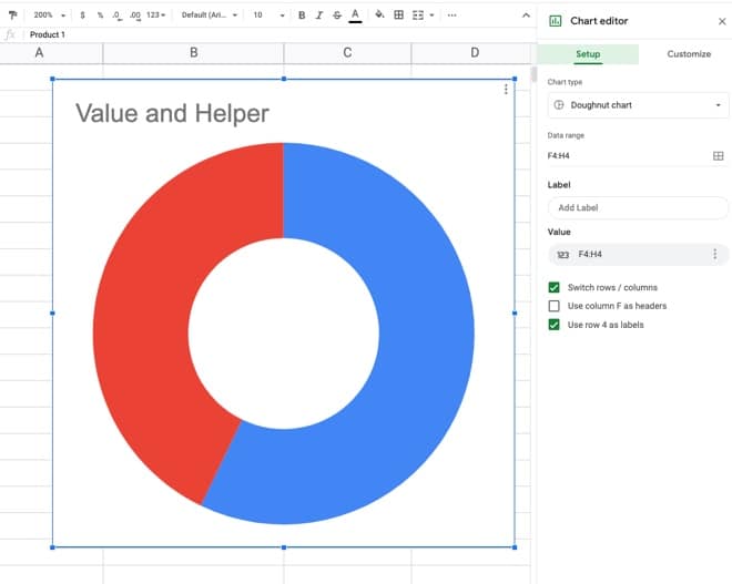
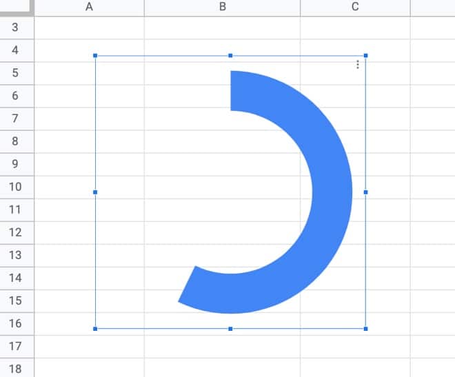
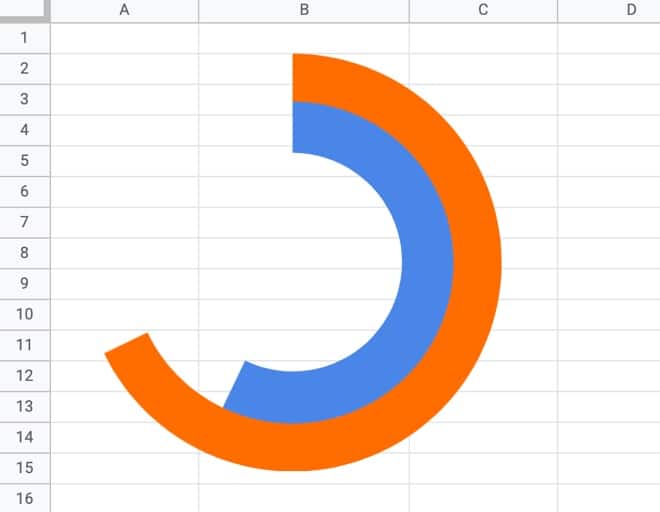
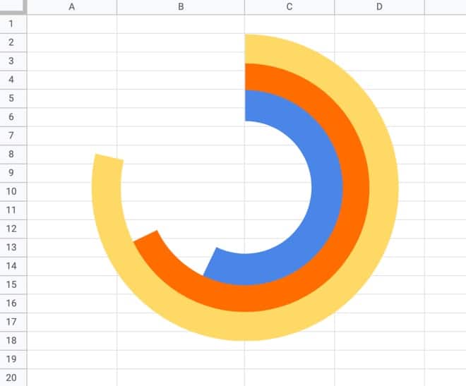
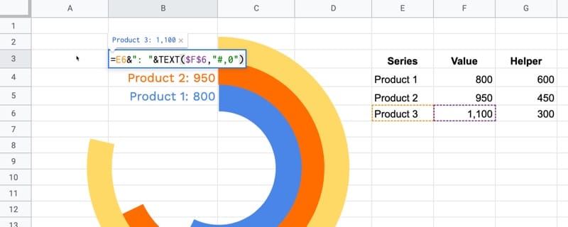
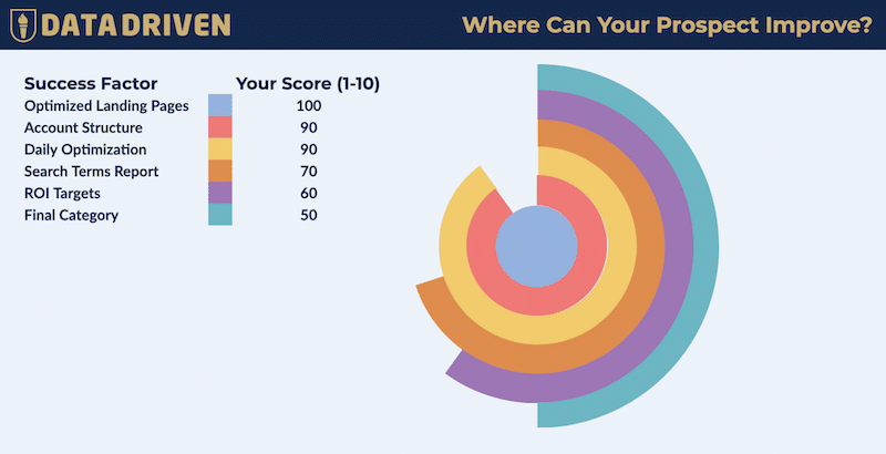


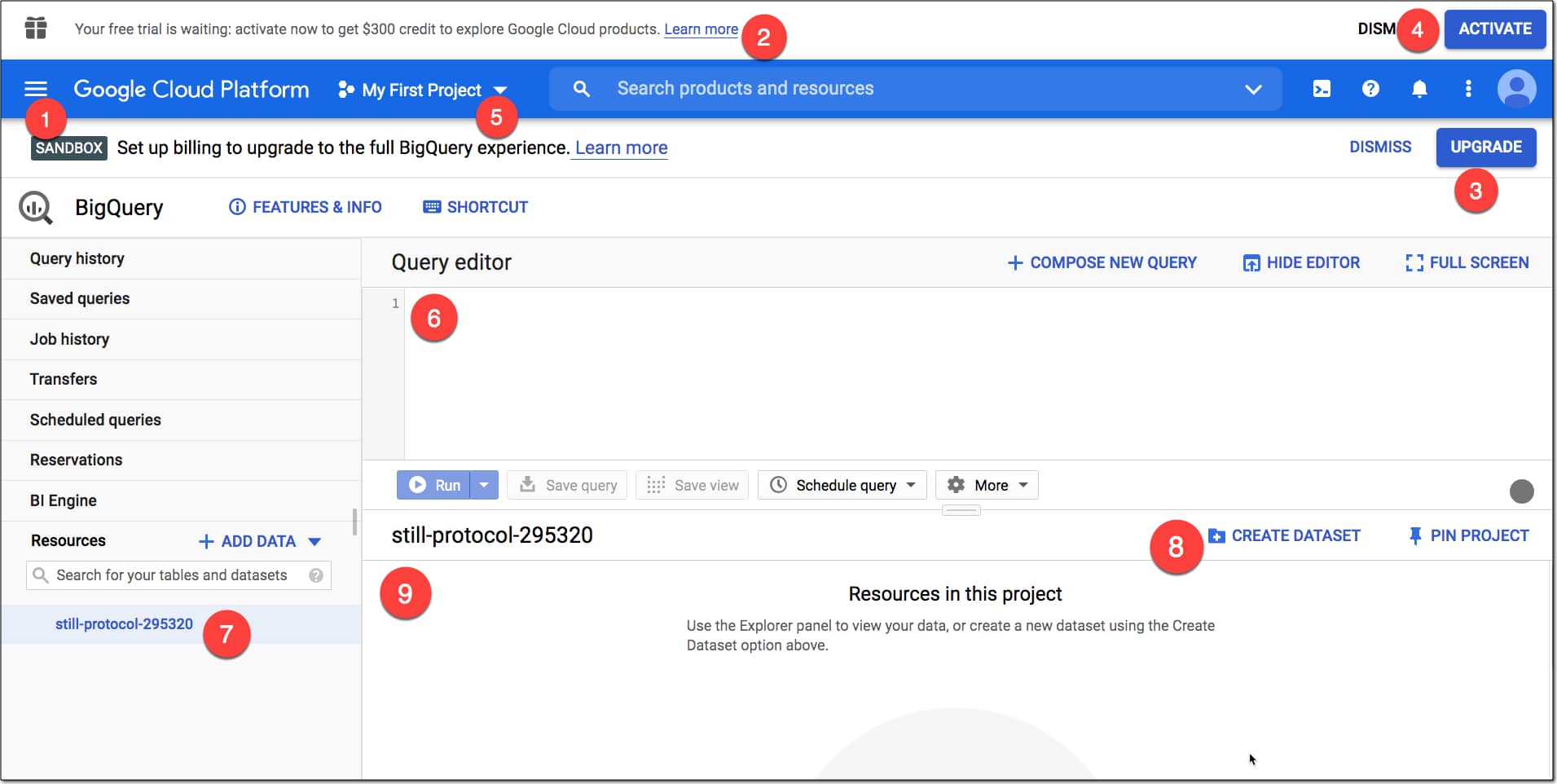
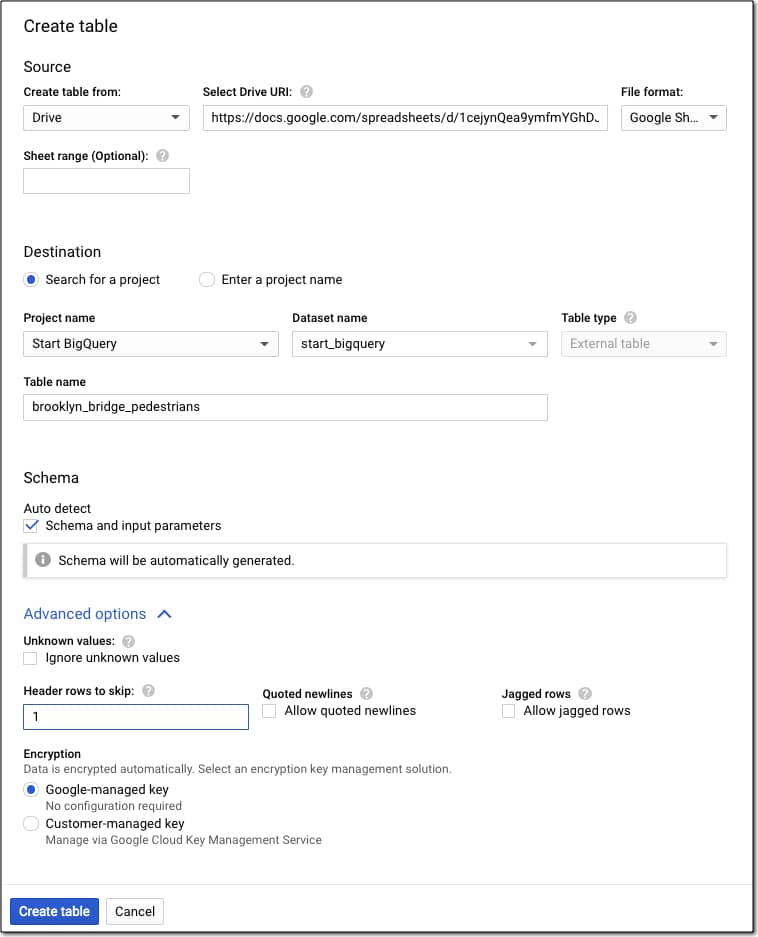
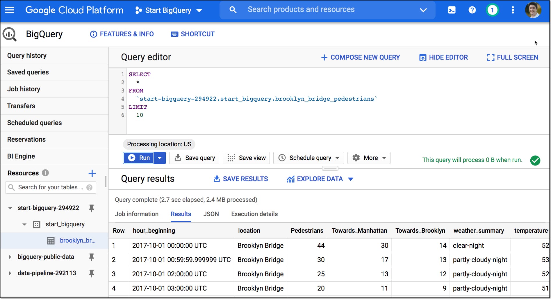
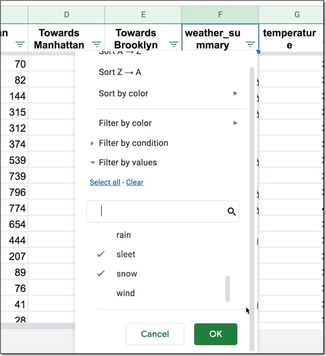
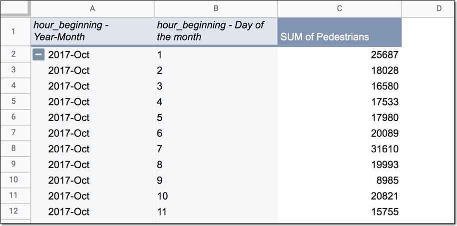
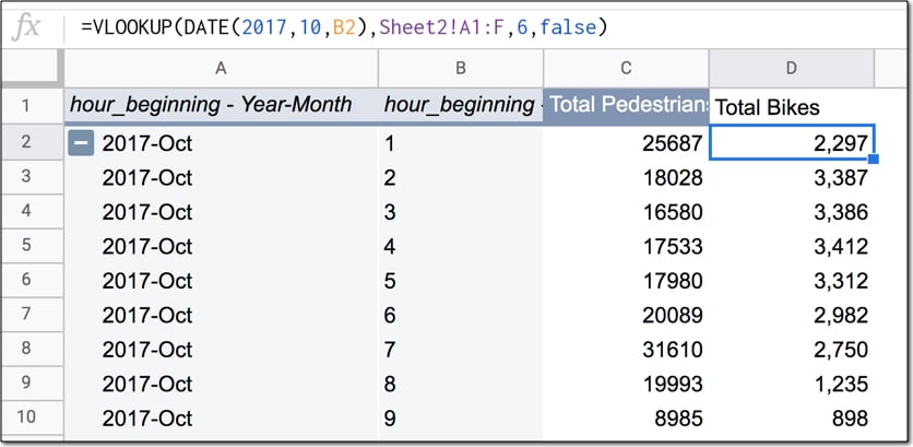
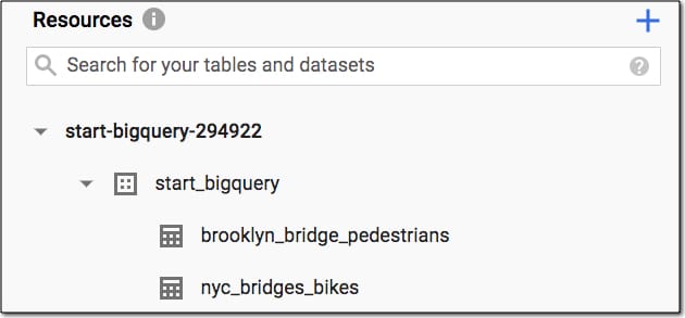
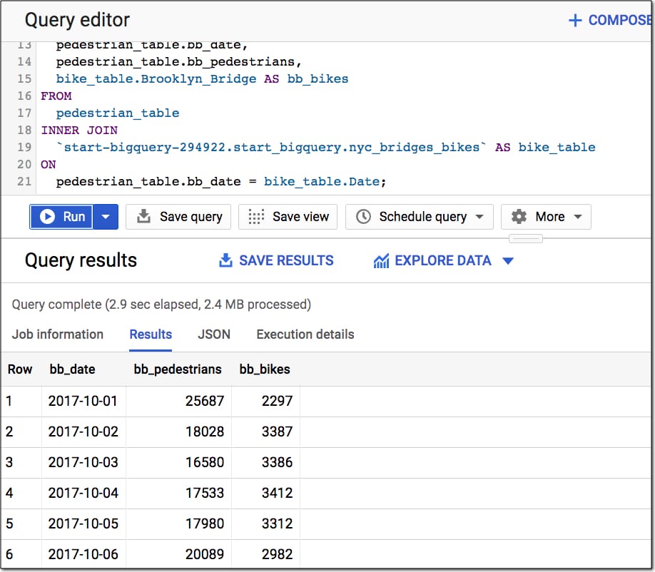
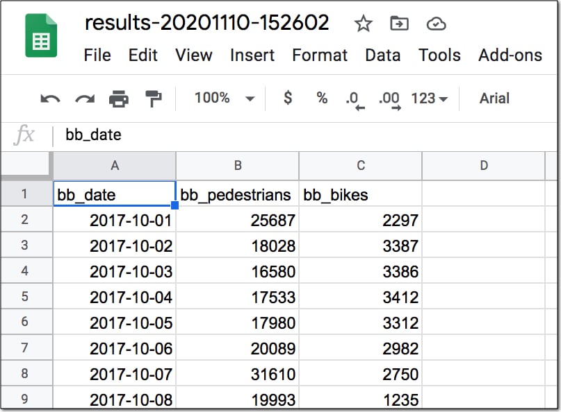
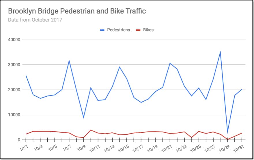


 1. How to use Google Sheets