This is a guest post from my wife Alexis Grant.
We use Google Sheets to solve all sorts of challenges in our family.
We combine Sheets with Tiller to track our family finances. We rely on a Google spreadsheet to stay on top of our home renovation project. And whenever one of us launches a digital product for one of our businesses, we build a dashboard in Google Sheets so we can watch sales in real-time.
Usually, when we build something fancy with Google Sheets, I need Ben’s help. But over the last few months, I used Google Sheets and a third-party tool to solve a problem I’d noticed in our town… and I didn’t need Ben’s help at all.
For this project, I used a no-code app builder called Glide. This was my first time using a no-code tool to build an app, and the first time I organized an app via Google Sheets. Here’s how I did it.
My no-code Glide App in Google Sheets: Hiking in Harpers Ferry, WV
Our family moved to Harpers Ferry, West Virginia, a year and a half ago. We decided to live here for access to hiking trails, and wow, has the town delivered on that promise. Several days a week, one or both of us leave our home at dawn for a walk in the woods or up the mountain.

Lots of tourists come to Harpers Ferry to hike, too. Yet there’s no one resource that outlines all the hiking options. The Harpers Ferry National Historical Park shares trails in the park. The Appalachian Trail Conservancy features local walks on the AT, and the C&O Canal Trust gives visitors local options, too.
But we couldn’t find a resource to share with visitors that combined all of these walks, plus others in town that don’t fall into any of these categories.
So I decided to build it.
I picked Glide because I’d heard about them at SheetsCon, Ben’s Google Sheets conference, where the company was a sponsor. I’d thought the concept was cool — an easy-to-use, web-based, drag-n-drop app builder that pulls data from Google Sheets. And it was free to get started.
In the end, Glide was as easy to use as I’d hoped, and the app I put together achieved just what I’d hoped.
You can access it at HarpersFerryTrails.com.
You can use it in a laptop web browser, but it’s really designed for mobile. Since it’s browser-based, you don’t have to use a lot of data to download the app; it simply pops up in your browser.
Below I’ll review more details on how Glide works and which features I used.
How to create apps with Glide App, the no-code app builder
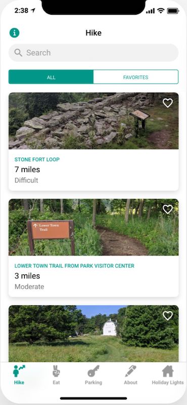
You can see in this screenshot of the app that it covers hiking Harpers Ferry, WV, as well as eating and parking.
While it took some practice to learn how to use the drag-and-drop interface, Glide was easy to use even for a first-timer. Here are the steps I followed to make an app with this no-code app builder.
1. Created the Google Sheets that power the app
All the information displayed in the app is housed in Google Sheets, so pulling that information together was the first step.
I created several tabs within my sheet, one each for hikes, restaurants, and parking. Then I added rows for each option and columns for details about those options.
For example, here’s what this looks like for the hikes tab:
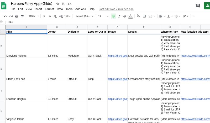
This was the most time-consuming part of making the app: gathering all the information and photos. Yet it’s also what makes the app truly useful.
2. Learned how to use Glide’s drag-and-drop interface
Next, I pulled that spreadsheet into my Glide account and fiddled with the settings to get each screen to look the way I wanted.
To adjust the information included in the app, I made changes to the spreadsheet. To adjust the presentation of that information, I changed items within the app itself, using different settings to choose various icons, titles, links, etc.
There was a bit of a learning curve since it was my first time using Glide, but the tool is generally user-friendly. In a few spots I had trouble figuring out how to do what I wanted, but with some poking around, I eventually accomplished it. I would have appreciated more tutorials or how-to instructions in Glide’s help community on how to accomplish specific tasks within the app; hopefully, they’ll build that out over time.
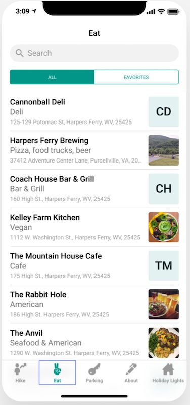
I liked how there were different ways to showcase the information, so I could pick the option that worked best for each screen. The restaurant screen below, for example, has shorter rows, while the hiking screen above shows a photo for each hike. Information can also be presented as a checklist, tiles, a calendar, and more.
Once I was happy with the Hike, Eat and Park tabs, I added an About tab to share some background on how the app came about and help users easily share it with their friends.
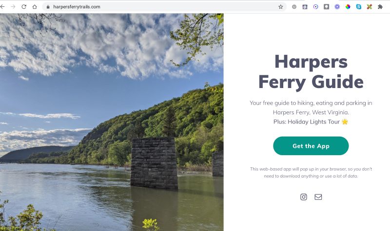
3. Built a landing page for my no-code app
Glide makes it possible to send new users directly to the app’s home screen. But I wanted a slightly different experience, a landing page that explained what to expect from the app.
As far as I can see, there’s no option to create this type of landing page within Glide itself, so I used Carrd.co to build a simple one-pager.
This particular landing page was incredibly easy to create; it only took a few minutes. The hardest part was getting my web host (MediaTemple) to point the URL, HarpersFerryTrails.com, which I already owned, to the Carrd.co site.
I love how simple and modern it turned out:
Carrd.co is not only easy to use, it’s also cheap. I upgraded to a $19/year pro account to use a custom URL.
4. Published the Glide app and asked for feedback
Once I published the app, I asked for beta users on Twitter and also had a few friends try the app.
I wanted feedback on whether the app was intuitive. Generally, the answer was yes, and I also received some helpful feedback that prompted me to make some tweaks.
(If you have any feedback you want to share, I’m all ears! Contact me here.)
Step 5: Help users find the app
Now I need people to use the app to navigate hiking, eating, and parking in Harpers Ferry! This is always the hardest part of creating anything online: helping the right people know about it.
While I’ve mentioned it to some residents already, I want to dedicate time and energy in 2021 to let people know this resource is available, and that it’s free.
One way I began to attract new users near the end of 2020 was by working with our tourism board to add a temporary Holiday Lights tab. They organized a driving tour that showcased holiday decorations, a socially-distanced way for visitors to experience the town this winter.
Since I’d already built this app, it was easy to add an additional tab showcasing the holiday lights driving tour. This was a win-win: the app made it easy for people to follow the route on their phone as they enjoy the lights, and people who tried the app for the lights tour might return to it later for hiking or restaurant information, and maybe share it with their friends.
The holiday lights tour screen defaults to a map view:
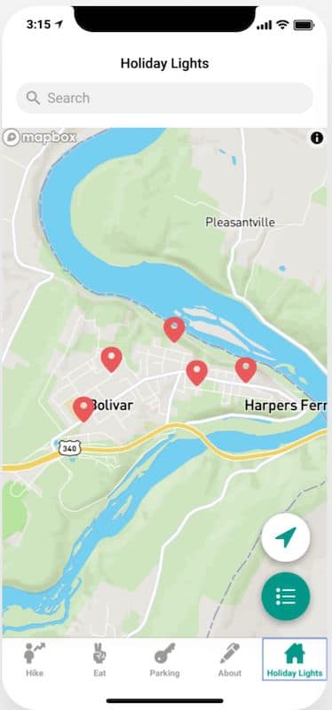
I wish there was a way to make this work more like a Google Map, with a route that shows the users’ location. I couldn’t figure out how to do that, so for this year, I kept it simple.
Now that the holiday lights tour is over, I can easily remove that tab from the app.
How to make apps for free: How much does a Glide App cost?
Because this isn’t a revenue-generating project and I plan to keep the app free for users, I didn’t want to spend much money to create it.
Glide made that possible: I used their free tier initially to create this no-code app. I was pleased from the get-go that the free tier provided everything I needed to make it functional.
However, there are a few features available with the paid version that later prompted me to upgrade to their lowest-paid tier:
- Map functionality. The free tier allows for a map, but only up to 10 locations. If you want to show more than 10 locations on a map, you have to upgrade to the paid version of Glide. Because we ended up adding more than 10 locations for the holiday lights tour, for example, I upgraded to the paid version to accommodate.
- Vanity URL. On the free tier, my app’s URL looks like this: https://ibo7l.glideapp.io/. That’s not easy to share or remember. With a paid upgrade, I could nab a custom, more memorable domain. That doesn’t really matter right now since I’m sending new users to the landing page at HarpersFerryTrails.com, but it could be a nice-to-have feature in the future.
- Creative icons. Glide’s free tier gives you access to a selection of basic icons, but you get more choices if you upgrade. Before I upgraded, for example, I had a peace sign for the Eat tab, because I didn’t have access to icons that were more food-related. Now all the icons feel intuitive.
When I wrote this post, here’s what the pricing tiers looked like:
- Personal app: Free
- Pro app: $32/mo or $24/year
- Private app: $40/mo + $2 per extra user
With paid tiers, you get more storage, more data rows pulled from your Google Sheets and more features. The company also offers business plans that charge according to how many users you have.
I’d really like to use their Google Analytics integration to see how many people use the app, but that feature isn’t included in the Basic plan, only in the Pro version. Since I didn’t have this feature during the holiday lights tour, I wasn’t able to see how many people actually used the app. (Another data point: We allowed people who drove the tour to vote for the best-decorated house through a Google Form, and we had more than 200 responses, which I suspect represents only a fraction of people who took the tour.) It would be fun to use Google Analytics to watch the user base for this app grow, so I might splurge for an upgrade in the future.
Glide is still just a few years old (founded by former Microsoft employees), so I won’t be surprised if their pricing options morph over time.
Conclusion
I never thought of myself as someone who would create an app or join the no-code movement. Yet this was enjoyable to build! Using Google Sheets as an organizational method felt natural and satisfying, and I appreciate that Glide allows me to iterate as I build, so the app is always improving.
Most of all, I’m happy to see the information I wanted to share available in a format that’s visual and easy to digest, which increases the benefit to users. I’m already scheming other ways to use Glide to create fun and useful apps, including an app that shows the schedule of events for a series of workcations I’m organizing called Retreat & Create.
These types of informational apps are really just the tip of the iceberg; you can also use Glide to build tools for your business, for example, an employee directory, applicant tracker, or inventory tracker.
Have you tried Glide or another no-code product that’s built on Google Sheets? We’d be keen to hear about your experience in the comments.
This post includes affiliate links, which means I get a small commission if you purchase a subscription via one of the links in this post.